International Journal of Civil Infrastructure (IJCI)

ISSN: 2563-8084

1. Introduction

Fiber-reinforced concrete (FRC) is a concrete with added discontinuous fibers to the cement, water, fine and coarse aggregate [1]. Fibers are added to concrete to improve its properties. Several fibers are used for this purpose: steel fiber, glass fiber, natural fiber, and synthetic fiber [2].

It has been proved that steel fibers improve concrete tensile and flexural strength [3], as well as the electric, magnetic, and heat properties [4]-[6]. Like steel fiber, Glass fibers improve concrete [7], while Synthetic fibers prevent plastic shrinkage cracks in fresh concrete [8]. Adding fibers to concrete has a much more significant effect on the flexural properties than on either the compressive or tensile strength [9]..

The addition of fibers in the concrete matrix increases the difficulty of studying the mixture properties and predicting the new mixture's behavior. But the experimental research showed that the primary benefit of fibers in the concrete matrix is the ability of the randomly dispersed and provide a crack arrest mechanism and enhance cracking performance. [10]. Therefore, the randomness of fiber is one of the most important properties to consider when modeling FRC.

Numerical modeling is a useful tool to represent the relationship between the microstructure and the mechanical or properties of materials. Finite Element (FE) modeling has been previously used to simulate FRC's behavior, but fibers are modeled as part of the concrete material [11, 12]. Such models do not present the randomness of fiber.

The objective of this paper is to provide an algorithm that accounts for fiber randomness in angle and location in the microstructure level of the material. The algorithm will then be used in Finite Element (FE) modeling. Since fibers have a greater effect on the concrete flexural properties than other properties, the algorithm and three-dimensional finite element model (3-D FEM) are used to calculate the flexural strength.

2. Algorithm to Generate Random Fibers

Fibers are distributed randomly in FRC regardless of the material used for fibers. It is necessary to create an algorithm to generate fibers randomly inside the specific domain; in this case, concrete beam, to capture an accurate material property for the concrete mixture. The resultant interaction between concrete and fiber in numerical modeling is highly affected by how accurate it can represent a random angle and location for the fibers.

MATLAB software is used to build the algorithm. In this algorithm, fibers are considered straight with a circular cross-section and with specific constant length, which in three dimensions (3D) makes one fiber a cylinder.

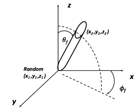
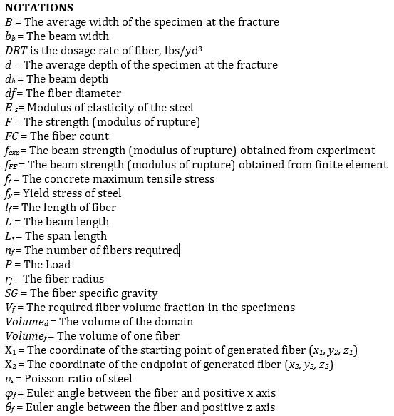
As shown in Figure 1, cylinder in 3D can be described by start point X₁ (x₁, y₁, z₁) and endpoint X₂ (x₂, y₂, z₂), radius (r_f ), length (l_f ), and two Euler angles (φ_f ) and (θ_f ) with positive x and z axes respectively.

2. 1. Generate One Fiber

The following steps are followed to generate one fiber randomly:

1. Generate the starting location of the fiber (X₁) randomly. In this study, the Mersenne Twister (MT) algorithm is used to generate a pseudo-random number list, developed by M. Matsumoto and T. Nishimura [13]. The generated point must be within the concrete domain.
2. Generate Euler angles (φ_f ) and (θ_f ) randomly, using MT algorithm that is used to generate the fiber starting point (X₁).
3. Calculate the second point (X₂). Where X₂ can be calculated using the following equation:

(1)



(2)



(3)


4. Check if the fiber second end X₂ is within the domain. If X₂ is outside the domain, step 2 will be repeated up to 10⁶ trials. if after that, the algorithm can't find a second point inside the domain, a new X₁ will be generated as in step 1

2. 2. Number of Fibers

The steps discussed are used to generate one fiber. But the algorithm will generate several fibers to satisfy the required fiber volume fraction in the specimens (V_f), where the number of fibers needed (n_f ) can be calculated using Equation 4. The number of fibers is rounded up to the nearest integer.

Where Volume_d is the volume of the domain. In this study, the domain is a beam. Therefore, Volume_d can be calculated using Equation 5:

Where d_b, b_b, and L are the beam depth, width, and length, respectively.

On the other hand,  is the volume of one fiber and can be calculated using Equation 6 as the following:

2. 3. Intersection

When mixing concrete with fibers, fibers do not intersect. It is essential to model the mixture by ensuring that fibers don't intersect in the domain. The criteria followed in this study to satisfy this condition is to generate a fiber with a minimum distance with all other fiber equal to twice the fiber radius (2r_f ). For each generated fiber using steps 1 to 4, the fiber minimum distance is calculated between the newly generated fiber and all previously generated fibers. If the condition is not satisfied, the newly generated fiber is rejected. The algorithm implemented here is the one used by Sunday [14]. The first step is to get the closest points for the infinite lines that they lie on. If they are in the range of the fibers segment, then they are also given the closest points. But if they lie outside the range of either, determine new points over the ranges of interest.

2. 4. Input and Flow Chart

All required rules are put together in one algorithm. The created algorithm inputs are related to the beam and fiber dimensions, which are usually predetermined. The following are the input for the algorithm:

• Fiber volume fraction (V_f)
• Fiber dimensions: radius (r_f ), length (l_f )
• Dimensions of specimens: d_b, b_b, and L are the beam depth, width, and length, respectively.

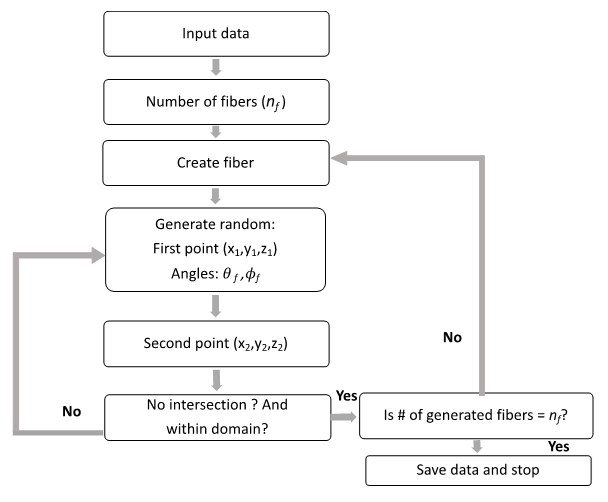
Figure 2 shows a flow chart that summarizes the algorithm. After the algorithm generates the required number of fibers, the program stops, and the data is saved in the output file. The output file includes the starting and ending points (X₁, X₂) for all random fibers. This data will be transferred to the Finite Element program to generate the geometry of the fibers.

3.  Algorithm Verification

To verify that the algorithm will generate a random fibers inside domain representing the real randomness in FRC mixture, the algorithm results are compared to experimental data in the literature. Stähli et al. have experimental research to study steel fibers orientation and distribution in concrete [15]. The study used CT-Scan to reconstruct a 3-D of the fiber distribution inside the concrete beam. 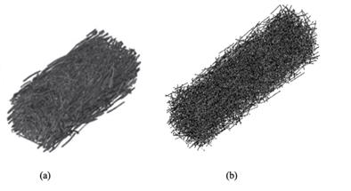The study's data are used in the proposed algorithm to generate the fibers, and the data is transferred to ANSYS [16] to visualize the section. The results are shown in Figure 3.  Figure 3-a shows the 3-D reconstruction of steel fibers in FRC from CT-Scan [15], and Figure 3-b shows steel fibers generated using the algorithm of the current study.

From the comparison, it can be seen the proposed algorithm can successfully model the mixture microstructure and achieved the randomness in generating fibers. This important aspect is required to model FRC.

3. 1. Flexure Behavior Testing

This section of the study focuses on the relationship between the microstructure and the mixture's mechanical properties. Since adding fibers to concrete has a much more significant effect on the flexural properties than on either the compressive or tensile strength [9]. The focus of this study is to use the proposed algorithm to model FRC flexural behavior. Fiber-Reinforced Concrete (FRC) flexural performance be tested Using Beam with Third-Point Loading based on ASTM C1609 [17].  The setup of the test is shown in Figure 4. A displacement is applied at a third distance, and load-displacement is monitored in the middle of the concrete beam.

Here, the target is to find the beam flexural strength or modulus of rupture (f ) using equation 7.

f: the strength (modulus of rupture)
P: the load
Ls : the span length
b: the average width of the specimen at the fracture
d: the average depth of the specimen at the fracture

3. 2. FRC Finite Element Modeling

Commercial FE software ANSYS APDL [16] is used to carry out the FE analysis using the appropriate elements and models for materials. Since this algorithm can be used with any fiber materials (Steel, Carbon, etc.), only materials used in this study will be discussed.

3.2.1 Element Types

Concrete is modeled using SOLID 65 element. This element is ANSYS concrete element with built-in cracking and crushing capabilities. All fibers are modeled as LINK 180; the element is a uniaxial tension-compression element with Tension-only (cable) and compression-only (gap) options [16] , which makes it suitable for different fibers material modeling. Any loading steel plates used in the study will be modeled as brick element SOLID 185.

3.2.2 Material Properties

Concrete material is modeled using a nonlinear uniaxial stress-strain. The model proposed by Kent and Park [18] is used to model the concrete behavior in compression. The concrete maximum tensile stress (f_t ) is calculated based on the ACI code [19] as:

Where f_c^' is the unconfined concrete maximum compressive strength.

Willam and Warnke's (1975) model [20] is used to define concrete's failure.

Any steel part will be modeled as elastic-perfectly plastic material. The yield stress (f_y), elastic modulus (E_s), and Poisson's ratio (ν_s) values depend on each individual study. Finally, composite polymers are modeled as a linear elastic material.

3.2.3 Mesh and Loading

Due to symmetry, a quarter of the test is modeled. The load is applied as an equivalent displacement at the top of the columns. Small mesh size is used to use shared nodes between concrete and fibers. The Full Newton-Raphson method is adopted to solve nonlinear equations, with a sufficient number of solution sub-steps during the loading process.

4.  Results and Discussion

The algorithm and Finite Element Model are validated by comparing the model results with experimental studies in the literature.  Three beams are chosen from three different studies: M2 [21], N4 [22], and  4PBT-small beams (Macrofiber) [23]. These beams are selected carefully to include a wider choice of fiber material and size, concrete strength, and beam size.

The verification included three steps:

1. Verification of the total number of fibers created.
   The total number of fibers in the beam is theoretically evenly distributed in the matrix, and with perfect dispersion, according to ACI 544.1R-96 [24]. It is calculated using equation 9.

(9)



Where FC is the fiber count, which is the number of fibers that theoretically occupy and are distributed in a unit volume of concrete matrix, d_f is the fiber diameter, DRT is the dosage rate of fiber, lbs/yd³, and SG is the fiber specific gravity. The total number of fibers FC_Total was found by considering the volume of the beam.
The results percentage of error (% Error) is calculated using equation 10.


(10)


2. The created fibers points are checked for randomness to ensure the quality of the model. MINITAB software is used to check for randomness using two tests:
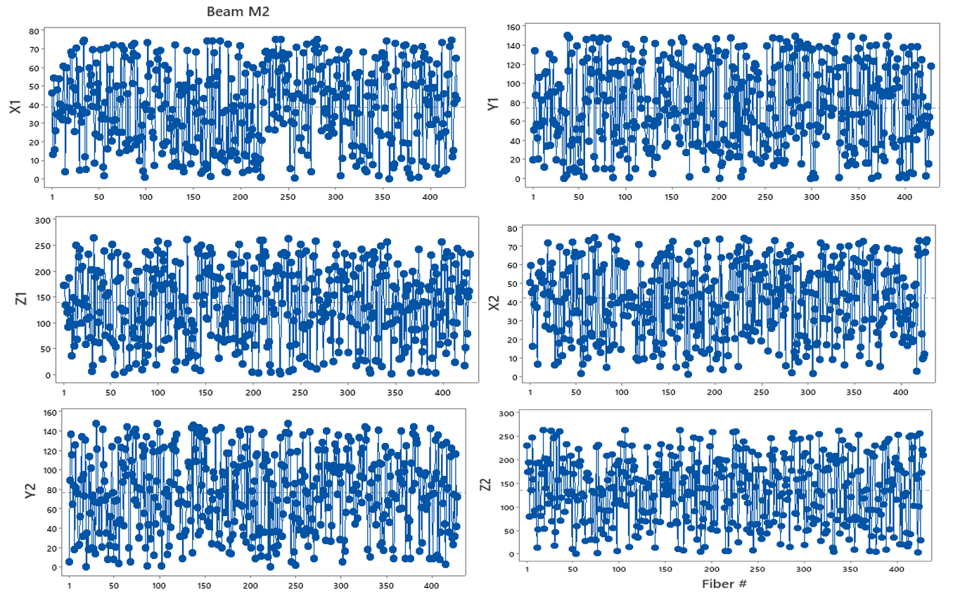
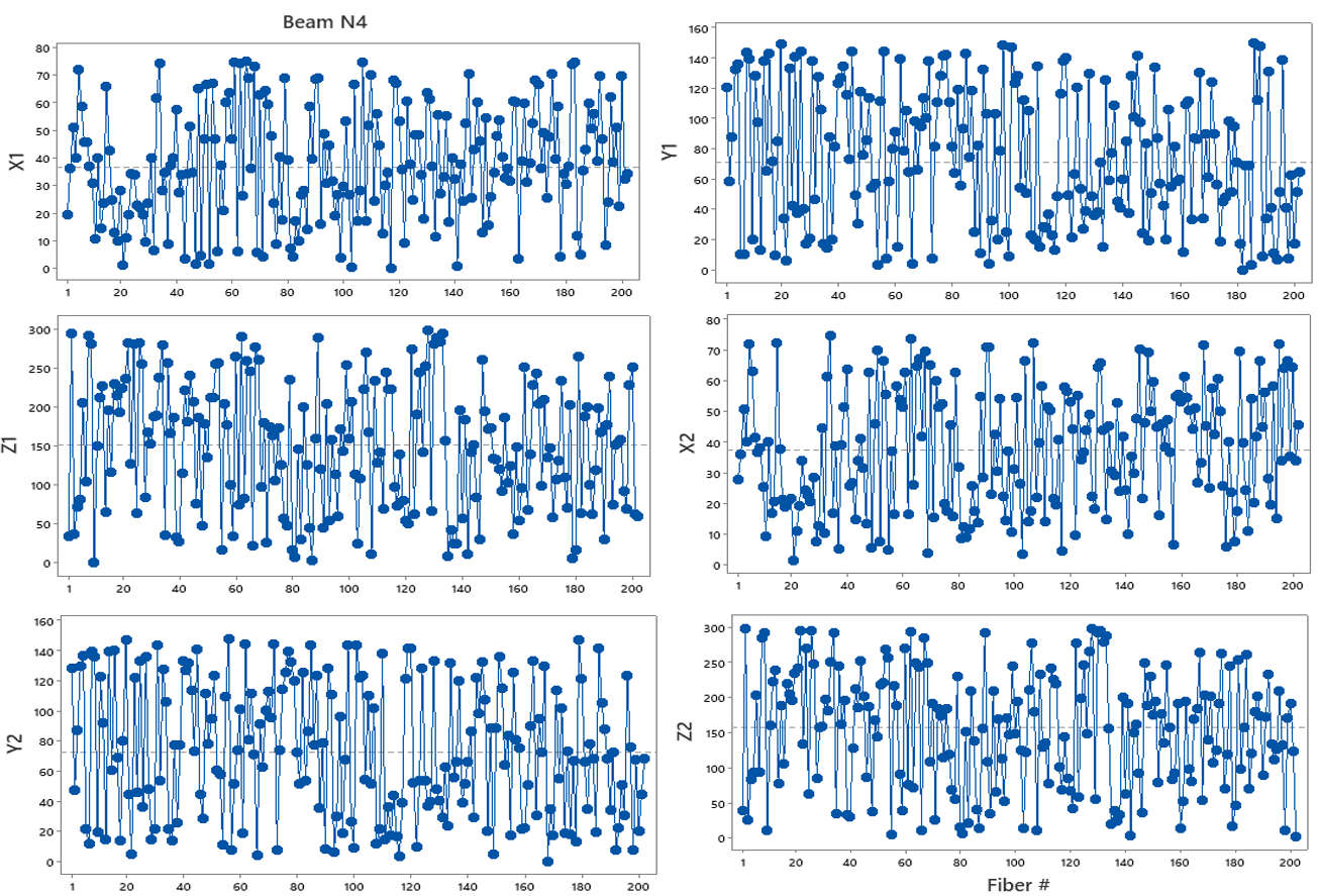
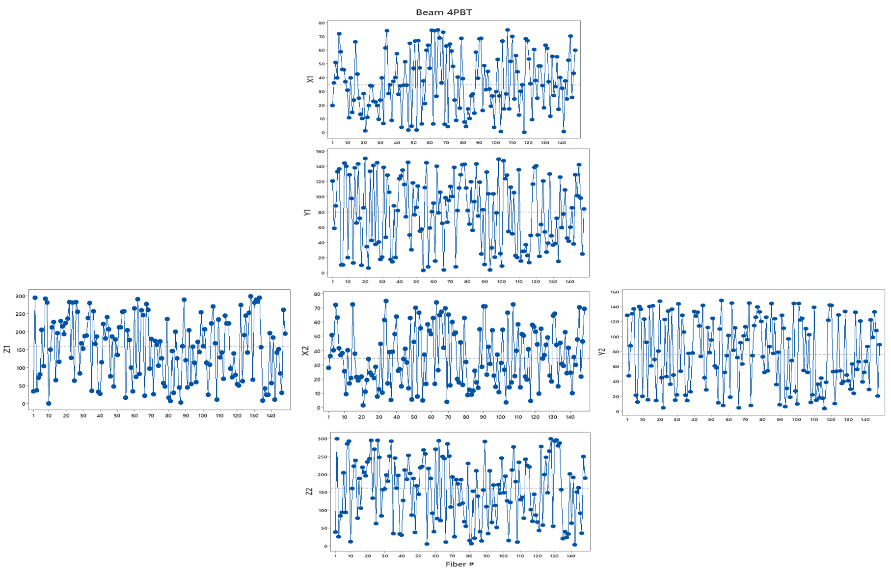
   Runs tests and Run charts are created for the fiber starting points (x₁, y₁, z₁) and the endpoints (x₂, y₂, z₂).
   Runs Test determines the randomness of data by comparing the observed runs to the number of expected runs.
   The run chart detects trends, oscillation, mixtures, and clustering of the data. Where trend is a drift in the data, either up or down, oscillation is the fluctuation of data up and down, Mixtures are characterized by the frequent crossing of the centerline, and Clusters are groups of points that have similar values [25].
3. Verification of the modulus of rupture. The experimental and FE values are compared.
   The results percentage of error (% Error) is calculated using equation 11.
   

   (11)
   
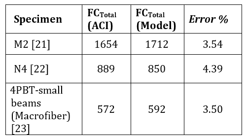
   The comparison between the algorithm generated the total number of fibers with the theoretical ACI number of fibers is shown in Table 1.
   The model overestimated the total fiber count for M2 and 4PBT by 58 fibers and 20 fibers, respectively. It also underestimated the fiber count for N4 by 39 fibers. Generally, there is a good agreement between the algorithm generated total fiber count, and the ACI total fiber count in the beams. The % Error ranged between 3.50 and 4.39, with an average of 3.81% error.

Table 1. Comparison between the Theoretical and model total fiber count

As discussed previously, the randomness of the created fibers is checked using the Runs tests and Run charts. The results of the Null hypothesis is that the order of the data is random, and the alternative hypothesis is that the order of the data is not random. The significance level of 0.05 is used. From that, a p-value of more than 0.05 will indicate the randomness of the data. Table 2 shows the p-value for the start and ending points of generated fibers.

Table 2. p values for fiber start and endpoints Run Test.

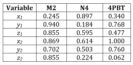
All variables have p, which is greater than the significance level of 0.05. accordingly, there is no evidence to conclude that the data are not in random order.

The second test is the run charts for all points (see Appendix A). The analysis's p values are listed in Table 3 for starts and endpoints of fiber for all investigated beams. The p values are obtained for trends, oscillation, mixtures, and clustering patterns. If the p-value for any of these trends is less than 0.05, data may have a nonrandom pattern.

From Table 3, all p values for all variables and patterns are more than 0.05. Therefore, no nonrandom patterns are detected in the created fibers.

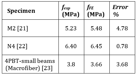
The finite element model using the created fibers is used to verify the beams' modulus of rupture. The experimental and FE values are compared.

Table 4 shows a comparison between experimental and Finite Element modulus of rupture Results.

There is a good agreement between the experimental and FE results. The % Error ranged between 0.78 and 4.78, with an average of 3.08%. Based on that, the algorithm and the finite element model can predict the FRC beam's flexural behavior with high accuracy.

Table 3. p values for fiber start and endpoints Run Test

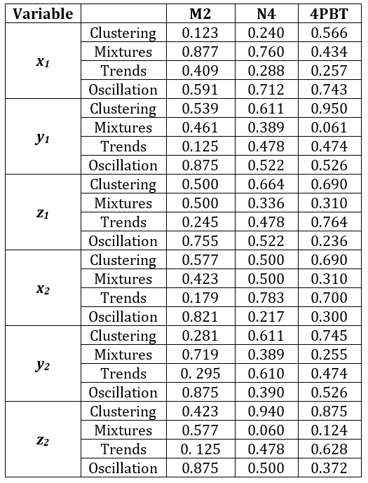
Table 4. Comparison between experimental and Finite Element modulus of rupture Results

Based on the results and the above discussion, the algorithm and the FE model can produce fiber in 3D random fibers and predict fiber-reinforced concrete's flexural behavior.

5.  Conclusion

This paper provides an algorithm that accounts for fiber randomness in angle and location in the material's microstructure level. The algorithm is used in Finite Element (FE) modeling to evaluate the fiber reinforced concrete beam's flexural performance.

The number of fibers created is in an agreement with ACI fiber count. The created fibers also show a high level of randomness.

There is a good agreement between the experimental and FE results, and the % Error ranged between 0.78 and 4.78.

The numerical simulations of the specimen under flexural loading agree well with test observations, which reveal that the algorithm and finite-element analytical approach can give reliable predictions.

References

Appendix A

References

[1] ACI Committee 544, "Guide for Specifying, Proportioning, and Production of Fiber-Reinforced Concrete," American Concrete Institute, Farmington Hills, MI, 2008.
[2] S. Yin, R. Tuladhar, F. Shi, M. Combe, T. Collister and N. Sivakugan, "Use of macro plastic fibres in concrete: A review," Construction and Building Materials, vol. 93, p. 180–188. DOI: 10.1016/j.conbuildmat.2015.05.105, 2015. View Article
[3] A. Beglarigale and H. Yazici , "Pull-out behavior of steel fiber embedded in flowable RPC and ordinary mortar," Construction and Building Materials, vol. 75,pp. 255-265 .https://doi.org/10.1016/j.conbuildmat.2014.11.037, 2015. View Article
[4] P. Sukontasukkul, W. Pomchiengpin and S. Songpiriyakij, "Post-crack (or post-peak) flexural response and toughness of fiber reinforced concrete after exposure to high temperature," Construction and Building Materials , vol. 24, no. 10, pp. 1967-1974, 2010. View Article
[5] Q. Dai , Z. Wang and M. Hasan , "Investigation of induction healing effects on electrically conductive asphalt mastic and asphalt concrete beams through fracture-healing tests," Construction and Building Materials , vol. 49, pp. 729-737, 2013. View Article
[6] Al-Mattarneh, "Electromagnetic quality control of steel fiber concrete," Construction and Building Materials , vol. 73, pp. 350-356. View Article
[7] S. Tassew and A. Lubell , "Mechanical properties of glass fiber reinforced ceramic concret," Construction and Building Materials, vol. 51, pp. 215-224, 2014.View Article
[8] M. Cao , C. Zhang C and H. Lv , "Mechanical response and shrinkage performance of cementitious composites with a new fiber hybri," Construction and Building Materials, vol. 57, pp. 45-52, 2014. View Article
[9] P. Song and S. Hwang, "Mechanical properties of high-strength steel fiber-reinforced concrete," Construction and Building Materials, vol. 18, p. 669–673. doi.org/10.1016/j.conbuildmat.2004.04.027, 2004. View Article
[10] Z. Xu , H. Hao and H. Li , "Mesoscale modelling of fibre reinforced concrete material under compressive impact loading," Construction and Building Materials, vol. 26, p. 274–288, 2012. View Article
[11] M. Islam, M. Khatun, M. Islam and S. Dola, "Finite Element Analysis of Steel Fiber Reinforced Concrete(SFRC): Validation of Experimental shear Capacities of Beams," Procedia Engineering, vol. 90, pp. 89-95 , 2014. View Article
[12] M. Özcan, A. Bayraktar, A. Shahin, T. Haktanir and T. Türker, "Experimental and finite element analysis on the steel fiber-reinforced concrete (SFRC) beams ultimate behavior," Construction and Building Materials, vol. 23, p. 1064–1077, 2009. View Article
[13] M. Matsumoto and T. Nishimura, "Mersenne twister: a 623-dimensionally equidistributed uniform pseudo-random number generator," ACM Transactions on Modeling and Computer Simulation (TOMACS), vol. 8, no. 1, pp. 3-30, 1998. View Article
[14] D. Sunday, "Geometry Algorithms," 2012. [Online]. Available: http://geomalgorithms.com/a07-_distance.html#dist3D_Segment_to_Segment. [Accessed 11 2017].
[15] P. Stähli, R. Custer and J. Van Mier, "On flow properties, fibre distribution, fibre orientation and flexural behaviour of FRC," Materials and Structures, vol. 41, no. 1, pp. 189–196. https://doi.org/10.1617/s11527-007-9229-x, 2008. View Article
[16] ANSYS, "Documentation for ANSYS. Version 17.2," ANSYS Inc, Canonsburg, PA, USA, 2016.
[17] ASTM, "Standard C1609/C1609M–12. 2012. Standard Test Method for Flexural Performance of Fiber-Reinforced Concrete (Using Beam With Third-Point Loading)," ASTM International, West Conshohocken, PA., 2012.
[18] D. C. Kent and R. Park, "Flexural members with confined concrete," Journal of Structures. Div., ASCE, vol. 97, no. 7, pp. 1969-1990, 1971.
[19] 3.-1. ACI, "Building Code Requirements for Reinforced Concrete," American Concrete Institute, Farmington, MI, USA, 2014.
[20] K. J. Willam and E. P. Warnke, "Constitutive models for the triaxial behavior of concrete," Proceedings of the International Assoc. for Bridge and Structural Engineering, vol. 19, pp. 1- 30, 1975.
[21] M. Hsiea and . T. C. Song, "Mechanical properties of polypropylene hybrid fiber-reinforced concrete," Materials Science and Engineering A, vol. 494, no. 1-2 , pp. 153-157, 2008.View Article
[22] N. Banthia and R. Gupta, "Hybrid fiber reinforced concrete (HyFRC): fiber synergy in high strength matrices," Materials and Structures , vol. 37, no. 10, p. 707–716, 2004. View Article
[23] L. Sorelli, A. Meda and G. Plizzari, "Bending and Uniaxial Tensile Tests on Concrete Reinforced with Hybrid Steel Fibers," Journal of Materials in Civil Engineering, vol. 17, no. 5, p. 519–527, 2005. View Article
[24] American Concrete Institute, "Report on Fiber Reinforced Concrete," ACI Committee 544 , 1996.
[25] Minitab, "Tests for randomness in a run chart," Minitab, LLC., 2019. [Online]. Available: https://support.minitab.com/en-us/minitab/18/help-and-how-to/quality-and-process-improvement/quality-tools/supporting-topics/test-for-randomness/. [Accessed 09 2020].