International Journal of Civil Infrastructure (IJCI)

ISSN: 2563-8084

1. Introduction

The coupled problems of fluid flow and heat transport in porous media, particularly those related to underground hydrology, have aroused great interest in recent times for their application in the field of geothermal, as can be seen in Di Sipio et al. [1] and in Barla et al. [2]. Their study has even led to the establishment by the scientific community of standard or benchmark problems that allow verifying numerical codes in this field since, in general, they have no analytical solution. Among these problems are those of Bénard, Yusa and Elder, discussed in Cánovas [3], which have given rise to numerous scientific publications. In all of them, temperature patterns or profiles are coupled to the velocity field, mainly because the flow equation contains a density-driven term.

However, when the temperature range of the problem is narrow and the velocity field is essentially imposed by an external pressure gradient or piezometric levels (with negligible influence of flotation) that would cause a regional flow, the problem, although simpler in its mathematical model, can be potentially very useful. The straight profile of temperatures that would occur in the absence of regional flow under stationary conditions, away from the water flow inlet boundary (resulting in a constant heat flow to the bottom), would be distorted and curved by the effect of the horizontal and vertical drags when there is regional flow. Thus, at all times, the temperature profile with depth is determined by the thermal properties of the ground and the value of the regional flow, apart from the influence of the thermal boundary conditions of the scenario. If, as it actually happens, the outside temperature is a seasonal function of time, its profile in the vicinity of the ground surface changes continuously, but its experimental measurement could allow the calculation of regional water flow. This is the objective of the present communication, to determine the connection between the underground water flow and the form of the temperature profiles that can be measured in a well. This would allow us to consider in the future the determination of the regional velocity field from the reading (direct and hardly expensive) of temperature profiles in wells.

The first approaches to this problem consist in investigating the shape of the temperature profiles in a 2-D scenario of sufficient extension, with constant regional flow in the horizontal direction and thermal conditions that reproduce approximately real cases, such as daily variation of the soil surface temperature and constant temperature at the bottom of the domain. In addition, different scenarios with vertical water flow are also studied.

For this study, a numerical model has been designed based on the network simulation method, whose reliability has been verified in García-Ros et al. [4] and in Cánovas et al [5]. The elaboration of the model is briefly introduced and it is applied to real scenarios to determine the characteristics of the correlation between the profiles obtained and the regional flows that determine them.

2. Nomenclature

Along this paper, the following example is employed to obtain and compare results according to the methodology presented in Harr and Eurocode. Figure 1 presents the geometrical variables of the modelled problem. That is, a sheet pile of a negligible thickness with a buried length in an almost infinite medium. Upstream and downstream the structure there is a water head difference that induces the groundwater flow.

	Capacitor
	Specific heat of the porous medium (Jm-3k-1)
	Thermal diffusivity (m2/s)
	Height or thickness of the porous medium domain (m)
JC	Current intensity flowing through a capacitor
JR	Current intensity flowing through a resistance
	Thermal conductivity of the porous medium (Jm-1s-1K-1)
	Horizontal length of the porous medium
Nx, Ny	Meshing reticulation
R	Resistance (Ω)
Rx,1, Rx,2	Elemental cell horizontal right and left resistance (Ω)
Ry,1, Ry,2	Elemental cell horizontal upper and lower resistance (Ω)
	Time (s)
	Temperature (°C o K)
	Temperature at the center of an elemental cell (° C or K)
	Temperature in the center right of an elemental cell (° C or K)
	Temperature in the center left of an elemental cell (° C or K)
	Temperature in the upper center of an elemental cell (° C or K)
	Temperature in the lower center of an elemental cell (° C or K)
	Temperature at x=0, x=L and y=0 (°C o K)
	Temperature at y=H (°C o K)
	Temperature at t=0 (°C o K)
	Water velocity in the in the X and Y spatial directions (m/s)
	voltage of a capacitor
	Voltage of a resistor
	Horizontal and vertical spatial coordinates (m)
	Temperature at the upper edge of the domain
	Elemental cells components
	Storage term in the heat flow equation in a porous medium (equation 7)
	Diffusive term in the heat flow equation in a porous medium (equation 7)
	Advection term in the heat flow equation in a porous medium (equation 7)
	Storage term in the heat flow different spatial finites equation in a porous medium (equation 8)
	Diffusive “x axis” terms in the heat flow different spatial finites equation in a porous medium (equation 8). Also called
	Diffusive “y axis” terms in the heat flow different spatial finites equation in a porous medium (equation 8). Also called
	Advection term in the heat flow different spatial finites equation in a porous medium (equation 8)
	Density of the porous medium (kgm-3)

3. The Physical and Mathematical Models

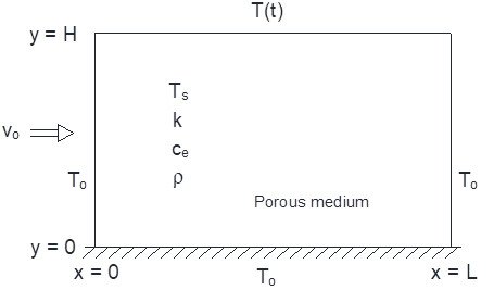
Figure 1 is a physical scheme of the scenario (with horizontal flow). As for the mechanical problem, a regional water flow induces a constant velocity field (vox) throughout the domain. As for the thermal problem (which assumes the phenomena of diffusion and convection in the porous medium), the following boundary conditions are imposed: i) constant temperature of the inlet fluid (first class or Dirichlet condition at the left vertical boundary, x=0), ii) seasonally time-dependent temperature at the upper horizontal boundary (special first class condition at y=H), iii) zero heat flow at the bottom (second class or Neumann homogeneous condition at y=0), and iv) constant temperature condition at the flow outlet front, x=L.

In order to eliminate the influence of the thermal flow output condition on the temperature profile, a sufficiently long horizontal domain has been adopted, reading these profiles in the previous region to the influence of this condition. The same precaution is taken regarding the influence of the fluid inlet temperature on the profile. These regions, before and after the profile measurement, depend on both the regional velocity and the thermal fluid properties.

3. References’ Solutions

3. 1. Harr Solutions

The mathematical 2-D model is formed by the following set of equations:

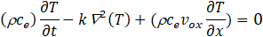
Where k is the thermal conductivity of the soil (Jm^-1s^-1K^-1), Ƥ the density (kg/m³) and cethe specific heat (Jm^-3K^-1).

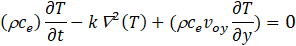
Eq. (1a) is that of heat transfer in the soil for the case of horizontal velocities. There is a diffusion in both spatial directions, a drag or convection in the OX direction and a local storage, quantities that are balanced in each volume or cell element. Temperature (T) is the dependent variable while spatial coordinates (x, y) and time (t) are the independent ones. For those scenarios with vertical velocity, Eq. (1b) is applied, in which case the drag or convection process is in the OY direction.

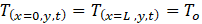
Eq. (2) represents the isothermal boundary conditions at the vertical sides x=0 and x=L of the domain, as well as eq. (3) at the bottom, and eq. (4) is the condition at the upper surface, where the temperature will be a function of time, T(t), approaching the seasonal variations of the environment.

Eq. (5) is the initial temperature of the soil and eq. (6a) or (6b) the solution of the flow velocity field at the domain. This is the model studied in this work although it is planned to extend it to more complex scenarios in future works. For example, velocity field dependent on depth, water table at levels below the soil surface, scenarios with sloping bottoms that imply the existence of vertical velocity components, convection and radiation incident fluxes on the soil surface, etc.

As we will see below, from the point of view of the network model design, these new scenarios do not entail special restrictions since the network method, discussed in González-Fernández [6] has successfully addressed problems of similar complexity, as can be seen in García-Ros et al. [4] and in Cánovas [5].

4. The Network Model

Taking those scenarios with horizontal velocity as reference, the network model is designed based on the finite-difference differential equation that derives from the spatial discretization of governing eq. (1a), retaining time as a continuous variable. For a volume element of an isotropic and homogeneous soil, this equation writes as

Where:

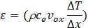
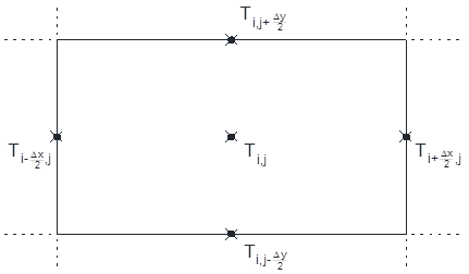
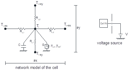
Now, we set the analogy between physical quantities ‘electric current ~ heat flux’ and ‘electric potential ~ temperature’. Using the nomenclature of Figure 2 for the volume element or cell, each addend of the former equation is assumed to be an electric current through a branch of the network (or electric circuit) that balances with the currents of the other addends in their respective branches in a common node. The voltage in this node, once the balance among currents is satisfied, is the temperature of the cell.

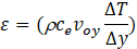
The constitutive equation between current and voltage through the electric component implemented in each branch must fit the mathematical expression of the related addend. Defining the soil thermal diffusivity (m²s^-1) and re-organizing the previous eq. (7), we have:

Where:

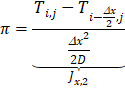
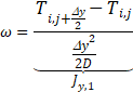
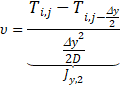
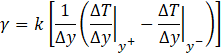
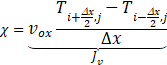
The current Jt is implemented by a capacitor of value C=1 since its constitutive equation is while the terms J_x,1, J_x,2, J_y,1, and _y,2, do it with resistors of value since the constitutive equation of such passive element is given by . Finally, Jv is implemented by a voltage-controlled current source (G), an active element of the circuit whose output, programmed by software, is given by the mathematical expression of J_v.

The network of the cell, shown in Figure 3, extends to the entire domain through simple ideal contacts between adjacent cells. Moreover, boundary conditions have to be added. Thus, vertical sides, eq. (2), are implemented by constant voltage sources, as well as eq. (3) in the bottom side, where in the upper side, eq. (4), a time-dependent voltage source is needed.

Finally, initial condition given by eq. (5) is implemented by charging the capacitors with an initial voltage of value T_s.

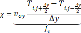
For those scenarios with vertical velocity (v_oy), the network model would be the same as shown before, with the only difference in the expressions (7.d) and (8.f), whose arguments would change to:

Once the model is introduced in a circuit simulation computer code, the free code Ngspice [7], it is run, giving the time-dependent solutions of the voltage (temperature) at all nodes and the currents (heat flux) at all branches.

Thanks to the powerful computing algorithms implemented in these codes, the simulation provides a practically exact solution of the model, relegating errors to the mesh size chosen. For meshes above 50x50 cells, computation times are low (5-30 s) and errors fall below 1%, a generally accepted value in engineering. This can be seen in Alhama [8].

5. Applications

Three different scenarios have been chosen. The first two are scenarios with horizontal water flow, while the third is for vertical flow .

5.1. First Scenario

The first one has the following data:

L= 40 m, H = 10 m, v_ox = 0.2 ms^-1, k = 1 Jm^-1s^-1K-1, = 2.7x10⁴ Jm^-3K^-1sup>, D = 2.7·10^-4 m²s^-1

T_o = 0 K, T(t) = 1 K, T_s = 0 K

N_x = 80, Δx = 40/80= 0.5 m, N_y = 20, Δy = 10/20 = 0.5 m, Simulation time = 1000 hours.

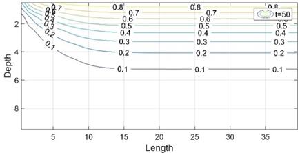
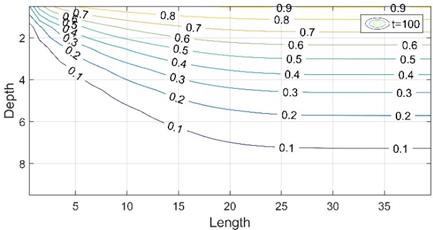
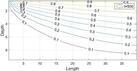
The simulation results, with a calculation time of around 20 s, are shown below. Thus, Figure 4 shows the temperature patterns for different simulation times. At 50 hours it can be seen that after about 20 meters from the left border, where the water flow comes from, a constant temperature profile is achieved, independent on the OX axis position. However, this is not a stationary situation, as we can see that at 100 hours the profile has evolved in depth (in this case the profile is more or less constant after 30 meters on the OX axis). It is around 500 hours when the stationary temperature profile is reached, since the thermal gradient is the same throughout the medium.

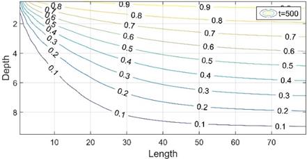
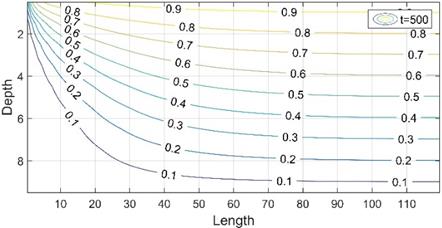
However, the distance on the OX axis to reach the stationary situation rises to 100 meters (Figure 5) for which it has been necessary to extend the length L of the problem to 120 meters.

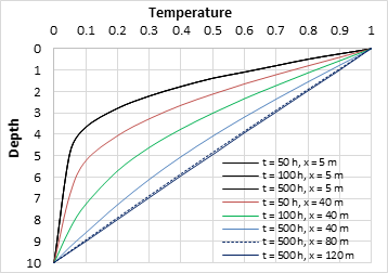
In view of these data it is observed how the temperature profiles, at times long enough for the stationary situation to be reached, are initially dependent on the position and then become independent in the central region. Figure 6 shows the different depth-temperature profiles obtained in the previous scenario, for different OX distances (5, 40, 80 and 120 meters) and for different times since the start of the problem (50, 100 and 500 hours).

This last profile (t = 500 hours) is the one that would be expected to be registered if in a field study we measure the evolution of the temperature with the depth in a borehole or well located in the considered OX position.

5.2. Second Scenario

The second scenario differs from the first in the following data:

L= 120 m, T(t) given in Figure 7, Nx = 120, Δx = 120/120= 1 m.

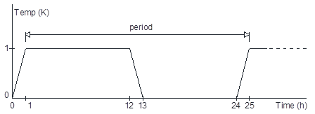
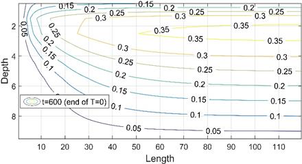
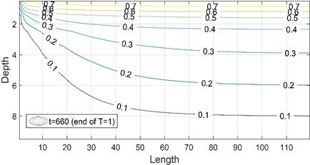
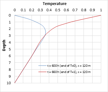
For this second scenario, the stationary situation is never reached, since the temperature varies periodically in the upper boundary. However, what does happen is that after approximately 600 hours have elapsed, the temperature patterns and profiles begin to repeat continually, as long as we compare them at the same time in the cycle or period. Thus, in Figures 8 and 9 the depth-temperature patterns and profiles are represented for the moments immediately before the beginning of the change of the temperature in the upper side (multiples of hours 12 and 24 hours, endings of T = 0 and T = 1, respectively).

5.3. Third Scenario

The third scenario corresponds to a case with vertical water flow and, initially, has the following data:

L= 40 m, H = 10 m, voy = 4·10^-6 ms^-1, k = 1 Jm^-1s^-1K-1, = 2.7x10⁴ Jm^-3K^-1, D = 1·10^-5 m²s^-1

T_o = 0 K, T(t) = 1 K, Ts = 0 K

N^x = 80, Δx = 40/80= 0.5 m, N^y = 20, Δy = 10/20 = 0.5 m, Simulation time = 3·10⁴ hours.

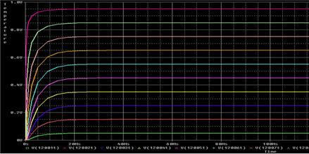
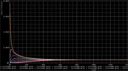
The simulation results, with a calculation time of around 15 s, are shown below. For this case, we illustrate the results from the output graphics of the Pspice [9] software, a code similar to Ngspice but with its own graphical interface. Thus, Figure 10 shows the evolution of the temperature for a column of soil (conveniently far from the lateral contours), in which can be observed how, after approximately 5000 hours, the steady state is reached. This can also be seen in Figure 11, where the evolution of the heat flow is represented for the different depths of the ground.

On this scenario, we will now present two interesting variants: in the first, once the steady state is reached, we will proceed to double the velocity, voy 8·10-6 ms-1, a change that we will make linear and progressive. In the second variant, once the stationary is reached as well, we will proceed to double the temperature of the upper edge, that is, T (t) = 2 K. These conditions are very easy to implement in the network method, in which it is only necessary to change the specifications of the parameters voy and T(t) at the desired time.

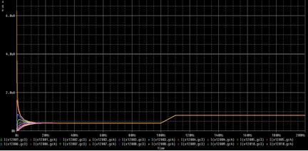
In the first case, it is observed how the heat flow doubles when velocity does, Figure 12, although this is not manifested in the temperature profile, which remains constant and looks identical to that of Figure 9. That is, the temperature field remains unchanged despite the fact that the total dragged heat has doubled.

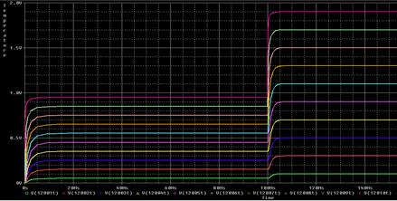
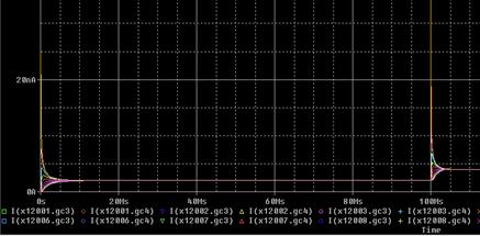
On the other hand, when we double the surface temperature the value of this variable is doubled in the whole domain, Figure 13, as expected. But in addition, it is also observed how the transmitted heat flow is doubled, Figure 14. However, for this last variable, it can also be seen how a second transient appears, a situation that did not happen in the previous case in which we doubled the velocity (Figure 12), where the increase in heat flow occurred linearly and gradually (remember that the change in velocity has been implemented in this way).

Conclusions

The network method has been successfully applied to different scenarios of heat transport within a porous medium through which underground water flows. Through this technique, different temperature boundary conditions have been implemented, so that simulated scenarios are very close to the reality observed in this type of problems.

The tendencies observed in the temperature patterns and profiles have provided very valuable information, since the lengths and the times in which the stationary, or quasi-stationary, state is reached have been determined, for both horizontal and vertical flow velocities.

The results obtained bring us closer to a horizon in which groundwater flux could be obtained from real field temperature readings.

7. Acknowledgements

We would like to thank the SéNeCa Foundation for the scholarship awarded to José Antonio Jiménez Valera, which will allow us to continue this investigation

References

[1] E. Di Sipio, S. Chiesa, E. Destro, A. Galgaro, A. Giaretta, G: Gola, and A. Manzella. "Rock thermal conductivity as key parameter for geothermal numerical models." Energy Procedia, vol. 40, pp. 87-94, 2013.View Artical
[2] M. Barla, A.D. Donna, and M. Baralis. "City-scale analysis of subsoil thermal conditions due to geothermal exploitation." Environmental Geotechnics, pp. 1-11, 2018.
[3] M. Cánovas. Caracterización adimensional y simulación numérica de escenarios patrón (Bénard, Yusa y Elder) de procesos geotérmicos de flujo y transporte. Doctoral dissertation. Universidad Politécnica de Cartagena, 2014.
[4] G. García-Ros, I. Alhama and J.L. Morales. "Numerical simulation of nonlinear consolidation problems by models based on the network method." Applied Mathematical Modelling, vol. 69, pp. 604-620, 2019.View Article
[5] M. Cánovas, I. Alhama, E. Trigueros and F. Alhama. "Numerical simulation of Nusselt-Rayleigh correlation in Bénard cells. A solution based on the network simulation method." International Journal of Numerical Methods for Heat & Fluid Flow, vol. 25, No 5, pp. 986-997, 2015.View Article
[6] C.F. González-Fernández. Applications of the network simulation method to transport processes, in Network Simulation Method. Ed. J. Horno, Research Signpost, Trivandrum, India, 2002.
[7] Ngspice – Open Source mixed mode, mixed level circuit simulator (based on Berkeley’s Spice3f5), 2016.Available: View Article
[8] F. Alhama. Solución de problemas lineales y no lineales de transferencia de calor por el método de simulación por redes. Doctoral dissertation. Universidad de Murcia, 1999.
[9] Pspice – version 6.0. Microsim Corporation, 20 Fairbanks, Irvine, California 92718, 1994.