International Journal of Civil Infrastructure (IJCI)

ISSN: 2563-8084

1. Introduction

In geotechnics and ground engineering, one of the most common aims is to control water flow both provisionally and permanently. In order to achieve this objective, retaining structures are built in the course of a river or a stream, or in excavations affected by water table. These structures can be concrete and earth dams, which are commonly thought to remain for a long time, or coffer dams, which are employed in sites to work in dry. However, whether building a permanent or a provisional structure, this must be designed according to different geotechnical phenomena (for example sliding, as happened in Aznalcóllar [1], or failure due to poor foundation soil, as in Saint Francis [2]), so it can be classified as safe. Among these phenomena is piping or heaving [3], a process that involves groundwater flow under the structure and leads to a situation that might not be steady and eventually end in failure.

As a mean to quantify the risk of pipping, two different values are compared: on the one hand, the estimated gradient, which depends on the geometry of the designed retaining structure and the piezometry under it (this can be studied with the flow net graphic); on the other hand, the critical gradient, which is a fictional number where the specific weight of the soil and the water are involved. When calculating the estimated gradient, theoretical universal solution graphics can be used [4]. However, these have been developed only for isotropic soils. Therefore, these solutions do not reflect the reality, since the majority of soils have an anisotropic behaviour.

Standards [5] also present methodologies to study whether the structure is safe or not, which depends on the estimated gradient and the total and the pore pressure in the most dangerous zones for this phenomenon. To employ this formulation, a deep knowledge of the process is needed, and this includes understanding the behaviour of the flow when running through anisotropic media.

In order to obtain all the necessary data to use formulations and compare results with theoretical ones, a methodology based on the network method [6] to simulate the flow through porous media under retaining structures has been developed. Network method is a simulation technique applicable to different physical phenomena, such as flow through porous media, soil consolidation [7], solute transport [8] and heat transfer [9]. This model employs the electrical analogy of the variables of the problem. That is, the equivalence of the groundwater head, h, with the electrical voltage, V, as well as the equivalence of the groundwater flux, Q, with the intensity, I. This is feasible since the governing equations in both cases are similar (constitutive equations). In this way, each cell in which the problem is discretized is transformed into a circuit with four resistors whose resistance values depend on the permeability of the medium, as well as the size of that specific cell. Once all the circuits are solved by using Ngspice [10], a specific free software for solving electrical circuits, the solutions are voltage and intensity for all the cells. From this, all the graphical and numerical results are obtained.

In this work, the risk of pipping and heaving is studied for a sheet pile structure in both isotropic and anisotropic media according to the estimated exit gradient obtained by Harr [4], the formulation presented in Eurocode [5] and our simulations. Therefore, the effect of anisotropy in the existing methodology can be observed.

2. Studied Problem

Along this paper, the following example is employed to obtain and compare results according to the methodology presented in Harr and Eurocode. Figure 1 presents the geometrical variables of the modelled problem. That is, a sheet pile of a negligible thickness with a buried length in an almost infinite medium. Upstream and downstream the structure there is a water head difference that induces the groundwater flow.

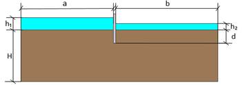
According to Figure 1 the dimensions are:
a: upstream length, in meters, 50.
b: downstream length, in meters, 50.
h₁: upstream water head, in meters, 5.
h₂: downstream water head, in meters, 0.
h: water head difference, h₁-h₂, in meters, 5.
H: stratum thickness, in meters, 50.
d: sheet pile buried length, in meters, 6.

When referring to the hydrogeological properties of the medium, they change if the soil is isotropic or anisotropic. For the isotropic medium, both permeabilities, k_x and k_y, take the same value, 0.1 mm/s, this is 10-⁴ m/s (which corresponds to a medium sand). Nevertheless, the anisotropic soil presents the same k_x but lower vertical one, 10^-6 m/s.

Finally, for both cases, the soil unit weight below phreatic level (γ _sat) is the same, 20 kN/m³, and with water unit weight (γ_w) of 10 kN/m³, effective weight unit (γ’ = γ_sat-γ_w) is 10 kN/m³.

3. References’ Solutions

3. 1. Harr Solutions

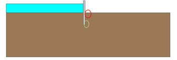
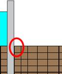
In ‘Groundwater and seepage’, Harr presents different universal graphics and equations to obtain the value of the exit gradient, I_E right after the retaining structure. In the example studied throughout this work, this gradient is calculated as shown in Figure 2 (red circle).

According to Harr, for this kind of structures, a universal solution exists for I_E, considering an isotropic soil, which is presented in Eq. 1.

Where I_E is the exit gradient, s is the sheet pile buried length, which has been previously named as d, and h is the water head different.

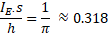
Therefore, the value of I_E for the problem here presented must be .

As the only solutions presented in this book are for isotropic soils, this value of I_E is later compared with the results obtained with the new methodology for both kinds of media.

The critical gradient, I_c, is defined as a comparison of the gravity forces of a submerged mass of soil (that is, the weight due to the particles minus the weight of the volume of water displaced by the soil particles), and the seepage forces in that same mass of soil due to the water flow. As the volume of the studied area is the same, this comparison is reduced to Eq. 2.

Where I_C is the critical gradient, γ’ is the effective weight unit, and γ_w is the water weight unit. According to the properties of the problem, I_c can be calculated as .

The safety factor for this phenomenon is then calculated as in Eq. 3

The safety factor according to Harr is 3.74. Nevertheless, this exit gradient is not the most harmful one for sheet piles structures, since the maximum gradients are found at the toe of the structure (I_T) on the downstream side (Figure 2, green circle).

In this way, Harr proposed a solution that involves the gradient in the whole buried length of the sheet pile, obtaining an average gradient in the area presented in Figure 3.

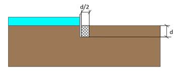
This method is the one employed for the study of heaving or piping phenomenon and the calculation of the safety factor of the sheet pile dam with the solution presented in this paper.

3. 2. Eurocode-7 Solutions: Verification against Failure of Hydraulic Heave

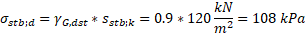
In this document, the stability of the structure is studied with two different equations. In both of them, destabilising actions are compared to stabilising actions in order to study the safety of the sheet pile. As the two kinds of actions are affected by a multiplier factor (partial factors presented in the Standard) that increase their value if they are negative actions and decrease it when they are positive ones, no safety factors are calculated. Formulations are those in Eq. 4 and 5.

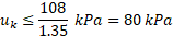
In Eq. 4, u_dst;d is the pore pressure (u_k) at the bottom of the structure (Figure 2, green circle) affected by a multiplier factor (γ_G,dst) that increases this value, as it is a destabilising pressure. For this example, γ_G,dst is 1.35, and u_k depends on the solution of the flow net and, therefore, should take a different value whether an isotropic or anisotropic medium is studied.

Still in Eq. 4, σ_stb;d is the stabilising total vertical stress (S_stb;k) at the bottom of the structure, again affected by a multiplier factor (γ_G,stb) that, in this case, decreases its value, since this is a stabilising pressure. Here, γ_G,stb is 0.9 and s_stb;k is a constant value for the problem, because it is not affected by the permeability of the studied medium. Therefore, according to Eq. 6

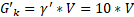
Thus, the value of the maximum admissible pore pressure uk can be obtained, according to Eq. 7.

In a similar way, Eq. 5 can be studied. Here, S_dst;d is the seepage force (S_k) in a soil column along the buried sheet pile length with an infinitesimal thickness, also affected by γ_G,dst, which increases this value. The seepage force, S_k, is calculated as the product of the average gradient along the pile length, which depends on the hydrology of the given problem (this is, if the soil is isotropic or not), the water weight unit and the volume of the fictional column of negligible thickness (V).

Also in Eq. 5, G’_stb;d is the submerged weight (G’_k) of this fictional column, affected by γ_G,stb, which decreases the stabilising force. G’_k keeps constant in this document, since the weight of the column does not change if the soil is isotropic or anisotropic. In this way, Eq. 8 is obtained.

Since V appears in both sides of Eq. 5, it can be removed, leading to Eq. 9.

From Eq. 9, the maximum value of the average gradient, i, takes the value presented in Eq. 10.

All in all, two comparisons must be carried out when employing Eurocode 7: the one involving the value of the pore pressure (Eq. 7), and another one, which obtains gradient (Eq. 10). Values u_k and i vary according to the problem, and even if the geometry is the same, solutions are different for isotropic and anisotropic soils.

4. Network Method Solutions

4. 1. Electrical Analogy

The Network Method is a technique to simulate different physical phenomena, including flow through porous media under retaining structures. This method is based on the electrical analogy, this is, making some or all of the variables involved in the studied problem equivalent to electrical quantities. In this case, the problem variables that are calculated are water head and water flux, which are equivalent to voltage and intensity respectively. This is feasible since the governing equation in both cases are equivalent, the only difference is the variables that are involved.

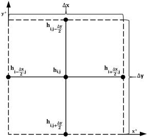
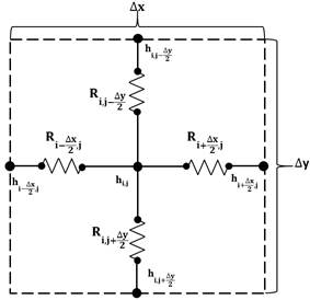
Therefore, the first step to employ this method is to discretize the problem geometry in cells. Each of these cells is transformed in a circuit with four resistors, two in vertical direction and two in the horizontal one, which resistance values depend on the horizontal and vertical permeabilities and the size of the proper cell due to the chosen discretization. Figure 4 shows the nomenclature of the elemental volume, while Figure 5 presents a typical circuit in the model.

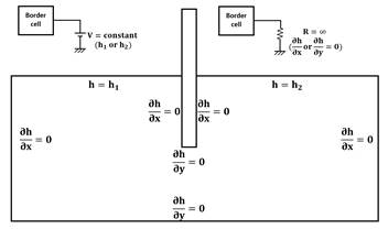
Moreover, boundary conditions must also be translated into electrical quantities. For example, impervious borders are simulated as resistors with very high resistance values (almost infinite), and the constant water head upstream and downstream the sheet pile are modelled in each of those cells with a battery which provides a voltage which is equal to the head value. In Figure 6, the boundary conditions are shown, as well as the devices modelling them.

Once all these data are transformed and the circuits are created, they are introduced in Ngspice, a specific software for solving electrical circuits. The raw solution of these are the voltage in each cell, as well as its vertical and horizontal intensity. In this way, as the equivalence with the problem variables is immediate, the values of water head and flux are obtained.

From the results, two different kind of solutions can be calculated:

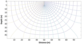
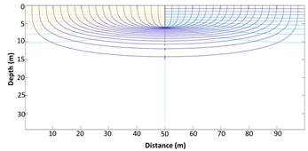
1) Graphical solutions, as flow nets, which show the behaviour of the water flow through the porous medium presenting the equipotential and the stream function lines. Figure 7 shows the flow net for the isotropic soil, while Figure 8 shows the same for the anisotropic problem. It is visible that, because of this lower vertical permeability, Figure 8 presents equipotential and stream function lines closer to the surface, since it is more difficult for the water to flow in the vertical direction.

2) Numerical solutions, such as total water flux or characteristic lengths. These are obtained by mathematical manipulation of the raw results provided by Ngspice. Among all these solutions, exit gradient (I_E), average exit gradient (i) and gradient at the toe of the structure (I_T) are the one of interest for this work.

4. 2. Results and Comparisons

Two values are obtained for each of the studied gradients, one for the isotropic soil and another one for the anisotropic medium.

The first comparison presented in this paper is the exit gradient according to Harr with the one obtained with the here presented network method. Previously shown here in Eq. 1, the value I_E is 0.265. Once the simulation for the isotropic example has been carried out, I_E turned to have a value of 0.258. This is very close to the theoretical one, taking into account that it is highly influenced by the discretization around the sheet pile, since I_E has been calculated in the upper cell closest to sheet pile in the downstream side, as shown in Figure 9 (marked with a red circle).

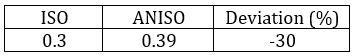
When simulating the anisotropic problem, however, this exit gradient value changes and goes up to 0.31. This shows that, when a lower vertical permeability appears, exit gradients tend to increase their values. If now the safety factors are calculated employing these two I_E obtained by the simulations, SF for isotropic problem is 3.88, while for the anisotropic problem this value is 3.23. In any case, according to this criterion, the studied sheet pile appears to be safe. Table 1 shows the theoretical and network method values of I_E, as well as the deviation between the theoretical and simulated values and between isotropic and anisotropic scenarios.

Table 1. Deviations for exit gradient (I_E).

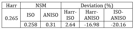
In Table 1, we can see that, as previous commented, the difference between the theoretical and the simulated value in the isotropic soil is soil is almost negligible. However, the deviation is remarkable when comparing any of the values for isotropic problem with that of the anisotropic soil.

Nevertheless, as also commented in this paper, this zone is not where the most harmful gradients appear. This can be demonstrated for the two presented examples. If instead of studying the cell in Figure 6, a similar calculation is carried out for the two cells at the toe of the structure in the same column, higher values of gradient are obtained for both simulations. For the isotropic soil, I_T takes a value of 3.81 (SF = 0.26), while this value is 3.44 in the anisotropic medium (SF = 0.29). If this criterion is followed, none of the cases seems to show a safe structure. Table 2 shows toe gradient values for both problems, as well as the deviation between them.

Table 2. Deviations for toe gradient (I_T).

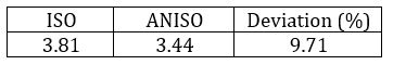
Table 2 shows how the anisotropy of soils affects the toe gradient, since the simulations have led to a difference of almost 10%.

Since both values, I_E and I_T, present such a difference, an average value is decided to be applied. In the proposed method, this value is calculated obtaining a gradient for each of the column of cells conforming the horizontal length d/2, and then calculating the average gradient of all of them. The gradient of each column (I_Cj) is calculated as presented in Eq. 11, and i in Eq. 12.

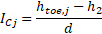
where h_toe,j is water head at the cell at the depth of the sheet pile and in the column number j, n is number of columns for d/2, and d_xj: horizontal length of the cell in columns number j.

Following the described calculations, the isotropic problem presents an average exit gradient, i, of 0.3 (SF = 3.36), while the anisotropic one has a value of 0.39 (SF = 2.57). Therefore, it is visible that, although in both cases the safety factor is greater than 1, the anisotropic option has a lower safety factor. The importance of considering the anisotropy of the soil is proved with the examples here presented. The difference between the values of i obtained with the simulation is presented in Table 3.

Table 3. Deviations for average gradient (i), first method

In this case, when considering a larger area where calculating the gradient, the effect of anisotropy is evident, with a deviation of 30%.

Taking up Eq. 6 and 7 when describing the methodology employed by the Eurocode-7, the values of uk and i must be calculated. For both variables, the water head in the cell next to the toe (h_toe) downstream the structure is needed. In the first example, h_toe = 2.1 m, while in the anisotropic one, h_toe = 2.219 m. Although these values are taken from the centre of the cell, not from the lower border, since the discretization is small, the position considered in the calculations is d. In this way, i is calculated as in Eq. 13

Therefore, for the isotropic example, i = 0.35, and in the anisotropic one, i =0.37. According to Eq. 10, in both cases the structure seems to be safe. The deviations, which, in this case would show the reliability of the retaining structure, are presented in Table 4.

Table 4. Deviations for average gradient (i), second method.

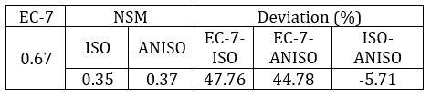
In this case, the comparison between the value obtained following Eurocode-7 and those from the simulations shows that the structure is very safe according to this methodology. Moreover, values of isotropic and anisotropic problems are very similar.

For the next verification, u_k must be calculated following Eq. 14.

In this case, for the first example, u_k = 81.00 kPa, while in the second one u_k = 82.19 kPa. So, both scenarios are slightly over the maximum value of pore pressure obtained in Eq. 7, presenting the anisotropic case the highest value. Table 5 presents the values of u_k obtained following Eurocode-7 and those from the simulations of the isotropic and the anisotropic scenarios, as well as the difference among them.

Table 5. Deviations for pore pressure (u_k).

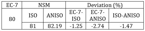
According to Table 5, the deviation between the theoretical values and those from the simulations is low (below 3% either in isotropic or anisotropic medium), and the difference when considering both conductivity ratios is even lower.

Results obtained from the indications in Eurocode-7 also show that, at least for the examples here presented, these would work whether isotropic or anisotropic soil is being considered. The percentages that have been calculated in Tables 4 and 5 corroborate so.

5. Final comments and conclusions

The use of the network method has led to the development of a numerical model for the simulation of the groundwater flow in isotropic and anisotropic soils. This tool gives the user the necessary information to study if retaining structures are geotechnically safe.

If the same structure is studied in an isotropic and an anisotropic medium, we can see that considering anisotropy is important for the determination of its safety, since the safety factors were lower for the anisotropic scenario.

Studying the toe gradient instead of the exit gradient leads to lower values of SF because piping is more likely to occur in this zone; nevertheless, since this would only happen in one point, employing the average gradient giver a more reliable idea of what is happening in a larger area.

Moreover, the use of the pore pressure instead of the gradient leads to safer solutions, as they seem more restrictive.

To conclude, whether isotropic or anisotropic is considered, Eurocode-7 seems to give accurate and safe results for piping process in retaining structures.

6. Acknowledges

We would like to thank the SéNeCa Foundation for the support given to this research and for the scholarship awarded to María Encarnación Martínez Moreno to carry out her doctoral thesis.

References

[1] A. Gens, and E. E. Alonso, “Aznalcóllar dam failure. Part 2: Stability conditions and failure mechanism,” Géotechnique, vol. 56, no. 3, pp. 185-202. 2006. View Article
[2] L. Begnudelli, L. and B. F. Sanders, “Simulation of the St. Francis dam-break flood,” Journal of Engineering Mechanics, vol. 133, no. 3, pp. 1200-1212, 2007. View Article
[3] R. Fell, C. F. Wan, J. Cyganiewicz and M. Foster, “Time for development of internal erosion and piping in embankment dams,” Journal of geotechnical and geoenvironmental engineering, vol. 129, no. 4, pp. 307-314, 2003. View Article
[4] M. E. Harr, Groundwater and seepage. Courier Corporation, 2012.
[5] CEN (2004) Eurocode-7 Geotechnical design - Part 1: General rules. Final Draft, EN 1997-1:2004 (E), (F) and (G), November 2004, European Committee for Standardization: Brussels.
[6] C. F. González-Fernández, “Applications of the network simulation method to transport processes,” Network Simulation Method, Ed. J. Horno, Research Signpost, Trivandrum, India, 2002.
[7] G. García-Ros, I. Alhama, and J. L Morales, “Numerical simulation of nonlinear consolidation problems by models based on the network method,” Applied Mathematical Modelling, vol. 69, pp. 604-620, 2019. View Article
[8] I. Alhama, A. Soto Meca, and F. Alhama, “Simulation of flow and solute coupled 2‐D problems with velocity‐dependent dispersion coefficient based on the network method,” Hydrological Processes, vol. 26, no. 24, pp. 3725-3735, 2012. View Article
[9] M. Cánovas, I. Alhama, G. García, E. Trigueros, and F. Alhama, F. “Numerical simulation of density-driven flow and heat transport processes in porous media using the network method”. Energies, vol. 10, no. 9 10(9), p. 1359, 2017. View Article
[10] Ngspice. (2016). Open Source mixed mode, mixed level circuit simulator (based on Bekeley’s Spice3f5). [Online]. Available: View Article