International Journal of Civil Infrastructure (IJCI)

ISSN: 2563-8084

1. Introduction

One of the most common objectives in geotechnics and ground engineering is the control of groundwater flow. For this aim, we can build retaining structures in rivers and excavations where a phreatic level appears. These can be coffer, earth and concrete dams, and they can be used as temporary or steady structures. They are also built with different materials.

If we focus on permanent concrete dams, the common studied variables are groundwater flow from the upstream side to the downstream of the dam and the pore pressure distribution under the structure because of this flow. This last variable is considered in a simpler way as the uplift force and its application point. The two phenomena are related to the safety study of the structure [1]. Large flow rates may be a risk at the dam toe, and pore pressure affects in safety calculations of overturning and sliding [2].

As a way to control both phenomena, sometimes one or serval piles are placed under the dam as part of the retaining structure. When they are employed, the flow rate is reduced, and there are variations in the values of uplift force and application point, depending these changes on the position and number of piles that have been located [3]. Some configurations have been thoroughly studied and analytical solutions have been obtained and presented in references manuals [4, 5]. However, these solutions only consider isotropic soils, leading to relatively reliable results, as most soils are anisotropic with lower values in the vertical direction.

Flow nets are another possible manner to study the variables of interest, as values of groundwater flow and pore pressure can be calculated from iso-potential and stream lines. Engineering manuals explain the rules to draw these nets, although these assume isotropic soils. Nevertheless, mathematical manipulations can be carried out to allow considering anisotropic media.

A third way to study these problems in isotropic and anisotropic soils is the use of software tools based on numerical methods. There are different options are available, and the one employed in this paper is the network method, which has already been applied in the study of different physical phenomena, such as flow in porous media [6], soil consolidation [7], and solute and heat transport [8, 9]. This methodology employs the electrical analogy, according to which, in this problem, the hydraulic potential, h, is equivalent to the voltage, V, and the groundwater flow, Q, to the electric current, I. This equivalence is correct because the governing equation in this problem and the electrical one are similar when they are spatially discretized.

According to this technique, each cell that is obtained by the discretization of the geometry is transformed into an electric circuit that has four resistors, whose resistance values involve the hydraulic conductivity and the cell size. When all the circuits are built, they are sent to Ngspice [10], a free software for solving electric circuits. Voltage and electric current values are obtained as solutions for all cells, and with these the results for the studied are built.

In this paper, we present the values of groundwater flow, uplift force and its application point for different scenarios of dam with a pile under it in different positions (heel, middle and toe) and without a pile, for an isotropic and for an anisotropic scenario. Therefore, the effects of the pile and the anisotropy can be studied.

2. Studied Problem

In order to compare the results obtained with the simulations, the same scenario is studied in all cases, according to the geometry of the medium and dam, as well as the hydraulic potential variation that generates the flow and, therefore, pore pressure distribution under the structure. Figure 1 shows the nomenclature of the common parameters of the scenario.

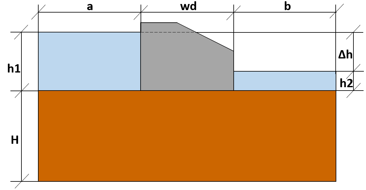
According to Figure 1, the main structure is a dam without a foundation, and the dimensions of the scenario are:

• a: upstream length, 50 meters.
• wd: dam width, 10 meters.
• b: downstream length, 50 meters.
• h1: upstream hydraulic potential, 10 meters.
• h2: downstream hydraulic potential, 0 meters.
• Δh: hydraulic potential change, 10 meters.
• H: stratum thickness, 20 meters.

Moreover, in the sheet pile scenarios, it has a length of 5 meters and a negligible thickness (10 cm in order to be able to run the simulation tool). The pile is located at 0, 5 and 10 meters measured from the dam heel for the scenarios of sheet pile at the dam heel, centre and toe.

Focusing on hydraulic conductivities in horizontal and vertical direction, the isotropic scenarios presents values of kx = ky = 10-5 m/s. However, anisotropic scenarios have values of kx = 10-5 m/s and ky = 10-6 m/s., this is, ten times lower. In both cases, the simulated media are clay sand, although anisotropic values are more realistic.

3. Network Simulation Method

3. 1. Electrical Analogy

The Network Simulation Method (or NSM) is a technique that allows studying different physical problems, and one of the possible phenomena that can be considered is flow through porous media under dams. The methodology is based on the electrical analogy, according to which the variables involved are equivalent to electrical quantities. For this problem, the groundwater flow is equivalent to the electric current and the hydraulic potential to the voltage. This is possible because the governing equations in both problems are very similar, and the only difference is the involved variables.

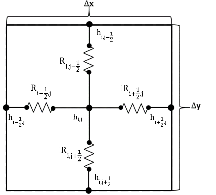
In this way, to start using the NSM, the geometry of the problem must be discretized in cells. Every cell is transformed into a circuit that presents four resistors, two in the vertical direction and two in the horizontal direction, and their resistance value depends on the hydraulic conductivity in each direction and the size of cell because of the chosen discretization. Figure 2 presents the nomenclature and typical circuit of an elemental volume.

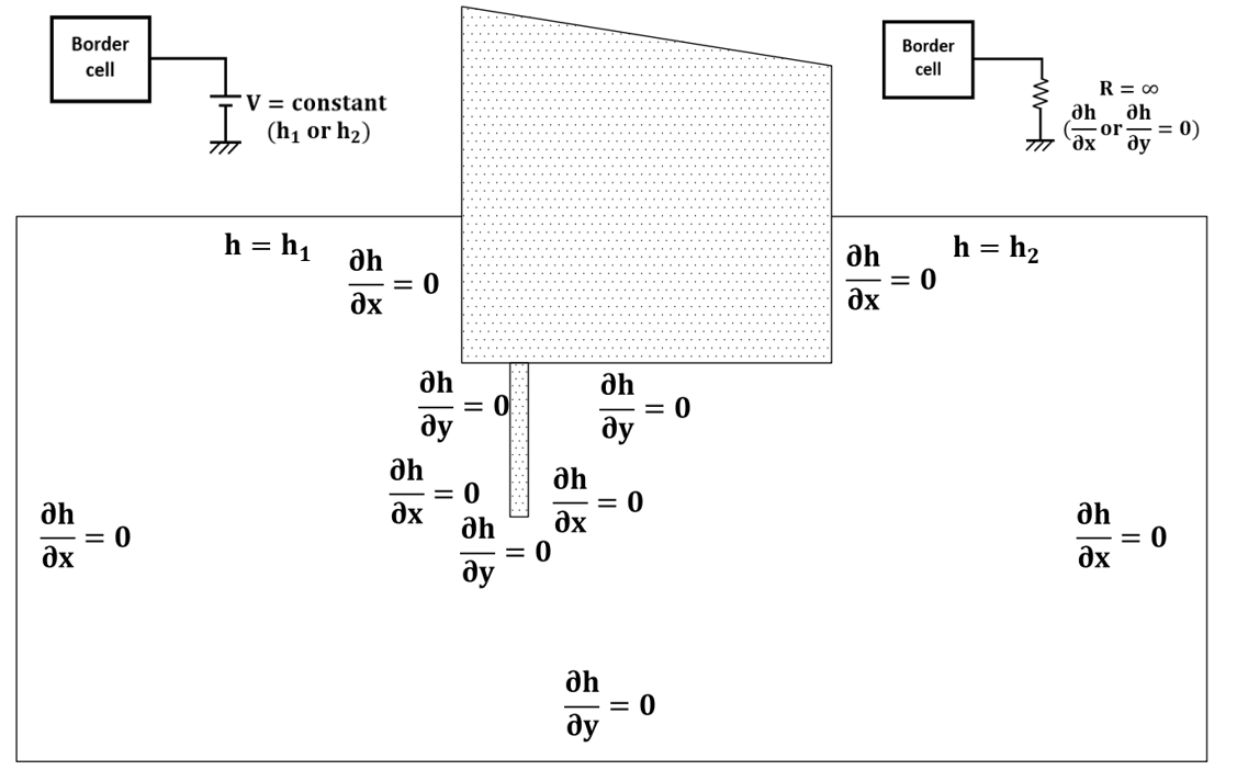
In addition, boundary conditions must be translated into electrical quantities too. For this problem, impervious borders are modelled as resistors of very high resistance value, almost infinite, and the upstream and downstream values of hydraulic potential are simulated with batteries whose voltage value is that of the potential to impose in that border. Figure 3 shows the boundary conditions and the suitable devices to model them.

3. 2. Results with the NSM

All the transformed cells and the electrical devices that model the boundary conditions are used by Ngspice to generate the whole circuit that simulates the studied scenarios once it has been solved. In this way, this software gives the values of voltage (or hydraulic potential) in all the nodes of the final circuit (commonly central nodes are employed) and electric current (or groundwater flow) in those branches that have been previously selected. With these values, the solutions of the problem are calculated, which can be of two kinds.

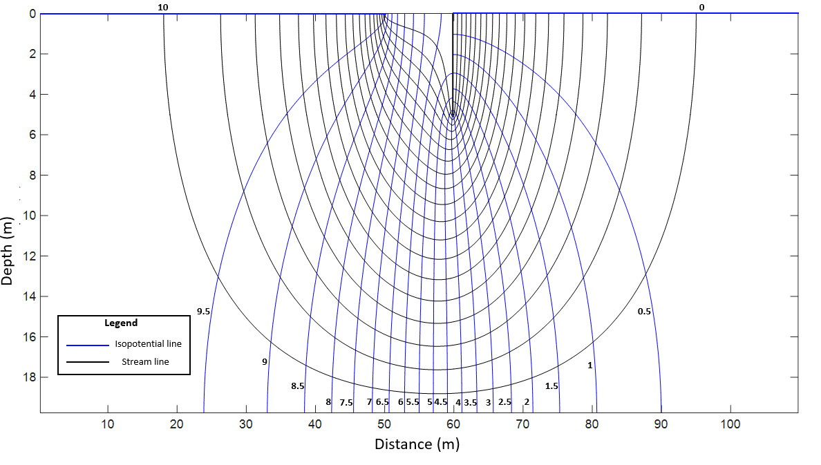
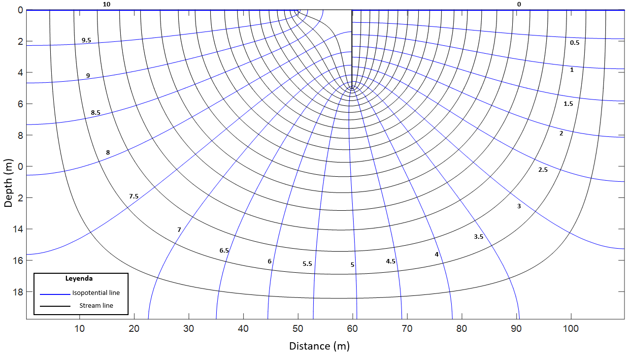
1. Graphical solutions, as the flow nets that the tool based on the NSM provides. These allow a good understanding of how the flow behaves under the dam and are different if the soil is considered as isotropic or anisotropic. The existence and location of pile under dam also alters the iso-potential and stream lines that are drawn in the flow nets. Figures 4 and 5 show those flow nets for scenarios of pile at the dam toe considering isotropic and anisotropic soils, respectively. With these, it is visible that, as the anisotropic scenario has a larger value of horizontal than vertical conductivity, the horizontal affected area (where most of the flow occurs) upstream and downstream the dam is larger than in the isotropic problem.

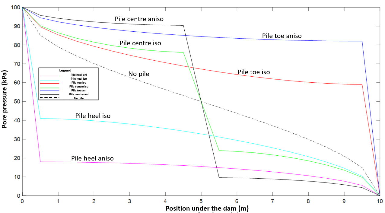
In addition, the pore pressure distribution under the dam can be also given as a graphical output, as shown in Figure 6. There, we see that when there is no pile, the pressure distribution for the isotropic and anisotropic problem have been presented as the same curve, so we can expect very similar values of uplift forces and application points for these two scenarios. When the pile is located at the toe, the pore pressure distribution has higher values for the anisotropic scenario, and the opposite occurs when the pile is at the dam heel, which means that higher values of uplift forces are expected in the first case if compared to the isotropic problem, and lower in the second case. Finally, placing the pile at the centre of the dam base makes the pore pressure distribution behave differently before and after the pile (following the flow direction) if anisotropy is considered. the values of the distribution are higher upstream the pile, and lower downstream when compared to the isotropic scenario.

2. Numerical solutions, which are obtained with mathematical calculations employing the results of Ngspice in all the cells as input information. Among all the possible results, those useful for this research are groundwater flow, uplift force and application point, although more variables can be obtained. Examples of these are the exit gradient right after the dam and the characteristic lengths, which is another way of measuring the zones through which most of the flow happens.

4. Results And Comparisons

As previously commented, in order to be able to compare the results, the geometry of the chosen scenarios is the same, and the only variations are the existence and location of the sheet pile under the dam. Therefore, as the same geometry is applied to isotropic and anisotropic scenarios, the effect of the anisotropy degree, A.D. –Eq (1)– and the equivalent hydraulic conductivity, k –Eq (2)– can be observed. These are useful parameters when two or more scenarios with different conductivities are studied: the combination of both allows quantifying the global permeability of the soil and how the horizontal and the vertical conductivities are related.

According to Eq (1) and (2) and employing the hydrogeological data presented in Section 2, for the isotropic cases, the anisotropy degree has a value of A.D.=1 and an equivalent conductivity of k=10^-5 m/s is taken, while the anisotropic examples have an A.D.=10 and a k=3.16 10^-6 m/s. As expected, the anisotropic soil is less permeable than the isotropic case, since the difference between the two kinds of scenarios is a lower vertical hydraulic conductivity.

Moreover, between the cases with and without sheet pile, since the only difference is its existence and location, results can also be compared.

4.1. Results Of The Studied Scenarios

Table 1 is a summary of the results of groundwater flow, Q, uplift force, F, and application point, C, for all the considered scenarios. In addition, in order to simplify the comprehension of the comparison of results presented in 4.2., the nomenclature of each scenario is also explained in this table.

Table 1. Nomenclature and variable values for all cases.

Name	Description	Q (m3/s/m)	F (kN/m)	C (m)
I.N.S	Dam in isotropic medium without a pile	7.40·10-5	500.10	3.73
A.N.S	Dam in anisotropic medium without a pile	3.23·10-5	500.10	3.75
I.S.H	Dam in isotropic medium with a pile at the heel	5.85·10-5	314.65	3.88
A.S.H	Dam in anisotropic medium with a pile at the heel	1.99·10-5	160.64	3.69
I.S.C	Dam in isotropic medium with a pile at the centre	6.23·10-5	500.03	3.26
A.S.C	Dam in anisotropic medium with a pile at the centre	2.03·10-5	500.03	2.82
I.S.T	Dam in isotropic medium with a pile at the toe	5.85·10-5	685.34	4.49
A.S.T	Dam in anisotropic medium with a pile at the toe	1.99·10-5	839.41	4.75

According to Table 1, some interesting results can be pointed out:

• The position in which the sheet pile is located must be thoroughly studied, since it can increase or decrease the uplift force (in isotropic scenarios the maximum difference is 370.69 kN/m, while for anisotropic scenarios this grows up to 678.77 kN/m). If other factors must be considered when deciding its location, a compromise solution must be chosen, in order to guarantee the safety of the structure from all the points of view considered in the project.
• Anisotropy must be studied employing both variables, anisotropy degree and equivalent conductivity, not only one of them, since, depending on the variable on which we are focussing, one or the other parameter becomes important.

4.2. Comparison Of The Studied Scenarios

In order to compare the results, this can be done in different ways when trying to reach conclusions. The effects of A.D. and k can be studied, as well as the effect of placing a sheet pile on the behaviour of the variables of interest. Finally, we can understand how the location of the sheet pile under the dam affects the problem.

4.2.1. According to anisotropy

The comparisons of results in order to study the effect of anisotropy is carried out according to Eq (3).

Where %Value_ISO-ANISO is the value of the comparison between isotropic and anisotropic results of the studied variables, Value_ISO is the isotropic value of the variable, and Value_ANISO is the value of the variable in the anisotropic scenario. The comparisons according to anisotropy are shown in Table 2.

Table 2. Comparison according to anisotropy.

Name	%Q	%F	%C
I.N.S-A.N.S	56.08	0.00	-0.54
I.S.H-A.S.H	65.98	48.95	4.90
I.S.C-A.S.C	67.42	0.00	13.50
I.S.T-A.S.T	65.98	-22.48	-5.79

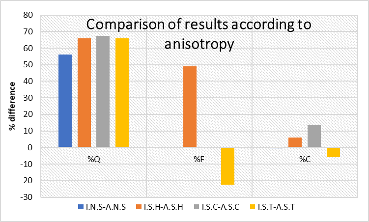
If the comparisons of groundwater flow are studied, it is observed that the variable decreases in anisotropic scenarios due to their lower equivalent conductivity, k. The difference is the same for %Q_I.S.H-A.S.H and %Q_I.S.T-A.S.T, which means that the values for the two configurations are the same, although this is better shown in the following comparisons.

Focusing on the comparison of uplift force, the variable is not altered because of anisotropy in scenarios without sheet pile (as previously commented) or with a sheet pile at the centre of the dam base (because the high values of pore pressure distribution upstream the pile are compensated with those of the downstream side). However, the uplift force decreases as the anisotropy degree increases if the sheet pile is located at the dam heel (because the values or the pore pressure distribution are lower), and the opposite occurs if it is at the dam toe (as the values of the pore pressure under the dam are higher).

Finally, the application point is hardly affected by the anisotropy degree for the scenarios of dam without a sheet pile (as has been explained in the previous section). Nevertheless, increasing the anisotropy degree, the value of the application point decreases when the sheet pile is located at the dam heel and centre of the dam base, moving towards the dam heel, and it is increased if located at the dam toe.

All in all, the variable that is more affected by anisotropy is the groundwater flow. Figure 7 summarizes the comparisons according to anisotropy.

4.2.2. Comparison between dam with a sheet pile and dam without a sheet pile

In this case, the values that are compared are those of the scenario without a sheet pile and those with a sheet pile in each location. In the same way, results for isotropic and anisotropic configurations are separately presented. The comparison is calculated as shown in Eq. (4):

In Eq. (4), %ValueNO-WITH is the result of the comparison of the studied variable between the value in the scenario without a sheet pile and that of dam with a sheet pile (different percentages for each position, H, C, or T of the pile under the dam), ValueNO is the value of the variable for the scenario without a sheet pile, and ValueWITH is the value of the variable if a sheet pile is under the dam. Table 3 presents the comparisons according to the existence of the pile.

Table 3. Comparison according the exitance of the pile.

Name	%QI	%QA	%FI	%FA	%CI	%CA
N.S-S.H	20.95	38.39	37.08	67.88	-4.02	1.60
N.S-S.C	15.81	37.15	0.01	0.01	12.60	24.80
N.S-S.T	20.95	38.39	-37.04	-67.85	-20.83	-26.67

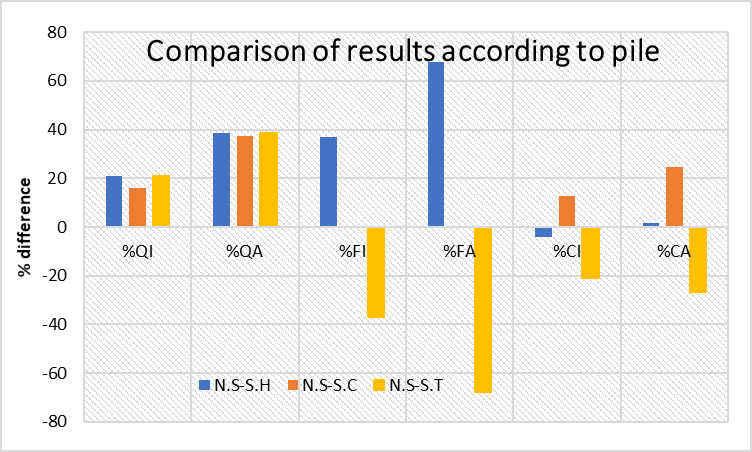
It is visible that groundwater flow variable is reduced when placing a sheet pile, either for isotropic or anisotropic scenarios. The reduction increases with the anisotropy degree.

The uplift force value is the same whether there is a sheet pile at the dam centre or without a sheet pile. It occurs in isotropic and anisotropic scenarios. If the sheet pile is located at the dam heel, the force is reduced if compared to that without a sheet pile because the values of the pore pressure distribution are reduced downstream the pile, and the opposite happens with the sheet pile at the dam toe, as the pore pressure values under the dam upstream the pile are increased.

Finally, the application point of the uplift force is not very affected when placing the sheet pile at the dam heel, independently of the anisotropy degree. If it is placed at the centre of the dam base, the value is reduced, and the reduction is more important as the A.D. increases because the pressure values upstream the pile are larger and those downstream are lower; and it is increased if the sheet pile is located at the dam toe.

In conclusion, the variable that is more affected by placing a pile under the dam is the uplift force. Figure 8 shows the comparisons according to the exitance of a sheet pile under the dam.

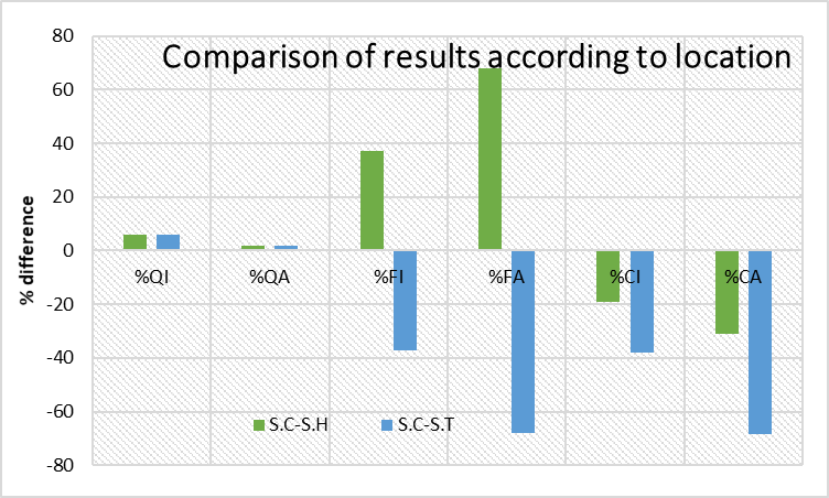
4.2.3 Comparison according to the location of the sheet pile

In order to carry out these comparisons, the base values are those of the sheet pile located at the centre of the dam base. Eq. (5) is employed for calculating these percentages.

In Eq. (5), %ValueCENT-EXT is the comparison between the value of the studied variable for scenarios of sheet pile located at the centre of the dam base and scenarios of sheet pile at the dam toe or heel, ValueCENT is the result of the variable for the scenarios of sheet pile at the centre of the dam base and ValueEXT is the value of the variable for the scenarios of the sheet pile at the dam heel or toe.

Table 4 summarizes the results of the comparisons according to the location of the sheet pile under the dam.

Table 4. Comparison according to the position of the pile.

Name	%QI	%QA	%FI	%FA	%CI	%CA
S.C-S.H	6.10	1.97	37.07	67.87	-19.02	-30.85
S.C-S.T	6.10	1.97	-37.05	-67.87	-38.08	-68.44

It is visible that the groundwater flow rate is the same when the sheet pile is located either at the heel or the toe, and it is lower than the rate generated if the pile is located at the centre of the dam base. This happens because the flow net behaves symmetrically with respect to the centre of the dam base.

We can observe again that the uplift forces for scenarios of sheet pile located at the heel and the toe are symmetrical with respect to the case of sheet pile at the centre of the dam base. The difference between values is larger as the anisotropy degree is increased.

Furthermore, the lowest value of the application point seems to occur if sheet pile is located at centre of the dam base (the point is closer to the heel), while the highest value is obtained if it is placed at the dam toe (it moves towards the toe). Figure 9 clusters all the results of these comparisons. The variable with the higher differences due to the location of the sheet pile is the application point.

5. Final comments and conclusions

The consideration of anisotropic soils in scenarios of flow under dams becomes relevant when searching for the values of the variables involved in safety analysis: groundwater flow, uplift force generated by pore pressure and its application point. Placing a sheet pile under the dam increases the importance of anisotropy.

Different scenarios have been simulated, in which the position of the pile is changed and anisotropy is considered or not. After the study of the most relevant configurations (pile at the heel, centre and toe of the dam), we have reached some conclusions. For those scenarios in which the pile is at the centre of the dam base, the uplift force takes the same value as if there was not a pile under it (500 kN/m), whether anisotropy is considered or not. Moreover, the amount of groundwater flow is reduced if employing the pile, and the lowest value is obtained in those scenarios where the pile is located at the dam heel or toe.

Locating the sheet pile at the heel o at the toe of the dam makes the scenarios behave symmetrically with respect to the centre of the dam base. That is the reason of groundwater flow differences when comparing the results of dam without a pile or with a pile at the centre are the same as for those where the pile is at one of the ends, whether the soil is considered isotropic or anisotropic.

The symmetry of the scenarios also affects the value of the uplift force, as it was visible, for example, when comparing the forces of the scenario where the pile is at the centre of the base to the other two problems with pile under the dam. In these cases, the differences take the same absolute value, since placing the pile at the dam heel decreases the uplift forces and the opposite occurs when it is placed at toe.

According to the geometry and hydrogeology presented in this document, in the isotropic problems there is a reduction of the flow rate of 16% when placing the sheet pile at the centre, and of 20% if it is at one of the edges. However, these reductions in the anisotropic scenarios are 37% and 38%, respectively. This means that considering realistic values of the hydraulic conductivities in both directions leads to larger reductions of flow rate.

Apart from reducing the flow rate, placing a sheet pile at the dam toe also leads to raise of the uplift force when compared to the values without a pile. In the examples presented in this document, the force and the application point are increased 37% and 21%, respectively, for the isotropic problems, while these values are 68% and 27% for the anisotropic cases. These results mean that a higher load is applied to the structure, and it is larger when anisotropy degrees higher than 1 appear, which is the common situation. If the design of the structure needs a sheet pile at the dam toe because other phenomena is also studied, the corresponding raise in the uplift values must be introduced in order to consider the most realistic scenario.

Finally, it was visible that the variable that is more affected by anisotropy is the flow rate, while the one with higher difference value when studying the effect of the exitance of a pile under the dam was the uplift force, and the larger differences appear for the application point when results comparing the position of the pile are observed. The numerical solutions presented in this document and the conclusions that can be derived are useful information to carry out safety analysis in dams.

6. Acknowledges

We would like to thank the SéNeCa Foundation for the support given to this research and for the scholarship awarded to María Encarnación Martínez Moreno to carry out her doctoral thesis.

References

[1] SPANCOLD. Instrucción para el Proyecto, Construcción y Explotación de Grandes Presas. 1967.
[2] CEN. Eurocode-7 Geotechnical design - Part 1: General rules. 2004.
[3] A. A. Ahmed and A. M. Elleboudy (2010). "Effect of sheet pile configuration on seepage beneath hydraulic structures", in International Conference Scour and Erosion (ISCE-5), San Francisco, CA, 2010, pp. 511-518. View Article
[4] M. E. Harr. Groundwater and seepage. Courier Corporation. 2012.
[5] M. Muskat. The flow of homogeneous fluids through porous media. McGraw-Hill Book Company. 1937. View Article
[6] E. Martínez-Moreno, G. Garcia-Ros, G. and Alhama, I. "A different approach to the network method: continuity equation in flow through porous media under retaining structures". Engineering Computations, vol. 37, no. 9, pp. 3269-3291. 2020. View Article
[7] G. García-Ros, I. Alhama and J. L. Morales, J. L. "Numerical simulation of nonlinear consolidation problems by models based on the network method". Applied Mathematical Modelling, vol. 69, pp. 604-620. 2019. View Article
[8] A. S. Meca, F. A. López and V. G. Fernández. "Density-driven flow and solute transport problems. A 2-D numerical model based on the network simulation method". Computer physics communications, vol. 177, no. 9, pp. 720-728. 2007. View Article
[9] M. Cánovas, I. Alhama, E. Trigueros and F. Alhama, F. "Numerical simulation of Nusselt-Rayleigh correlation in Bènard cells. A solution based on the network simulation method". International Journal of Numerical Methods for Heat & Fluid Flow, vol. 25, no. 5,pp, 986-997. 2015. View Article
[10] Ngspice. (2016). Open Source mixed mode, mixed level circuit simulator (based on Berkeley's Spice3f5). [Online]. Available: View Article