1. Introduction

Permafrost degradation, driven by global warming, is correlated to the increase in collapses which has been recently observed at altitudes above 3000 m asl. To name a few, the Brenva (2x10⁶ m³) and Punta Thurwieser (2x10⁶ m³) rock/ice avalanches in the Italian Alps [1], the rock/ice avalanche (3x10⁶ m³) at Bondo in Val Bregaglia, and the ice/debris avalanche (3x10⁶ m³) that occurred last summer on the Marmolada glacier in the Dolomites. In fact, although it is difficult to establish a direct trigger-effect relationship for any individual case, instabilities tend to occur more frequently during particularly warm summers, of which year 2003 represents the first explicit occurrence. It is also important to recall that collapses occur at altitudes close to the boundary of permafrost in alpine areas. In fact, the temperature of alpine permafrost in Europe has increased by up to 1.5 °C in the last century and this this corresponds to an increase in altitude of the lower permafrost line of about 100 m ([2], [3])

From a mechanical point of view, the warming of permafrost reduces the shear resistance along rock joints by triggering a number of adverse factors ([3], [4]), such as the decrease of ice resistance with temperature, water pressure increase and alteration of the creep properties of ice infillings. Moreover, repeated freeze-thaw cycles are responsible of fracture propagation. In this context, it is equally important to investigate and describe the mechanical behaviour at the scale of materials and joints, and to set-up numerical models at the scale of the rock mass that account for the stress-displacement joint behaviour.

1.1. Research framework

A multi-scale approach to improve the understanding and assessment of rock slope stability conditions in high mountains has been recently proposed [5]. Previous research at the material scale (ice and frozen soil, [6]) allowed defining an original failure criterion for continuous [7] and discontinuous [8] rock joints filled with ice (joint scale). This criterion can then be used in large scale DEM modes of rock masses, as it will be shown in this paper.

1.2. Study case

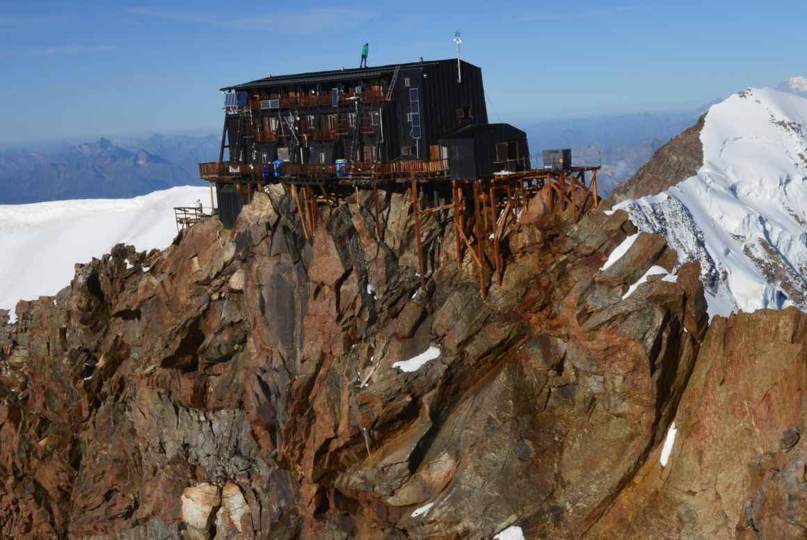
In this paper, the described approach is applied to the evaluation of the stability of Punta Gnifetti (Signalkuppe) in the Monte Rosa group. In particular, at 4554 m asl Punta Gnifetti is the fourth highest peak in the range. More interestingly, Capanna Margherita hut, the highest one in the Alps, is located just on the top of Punta Gnifetti (Figure 1). It is worth noting that the Monte Rosa group is among the areas most affected by the rise in temperatures during the last century.

The procedure adopted in the numerical simulations is based on a geomechanical based back-analysis [9] and the assumption of two different scenarios of rock-mass degradation (fracture propagation and temperature increase). Both back-analysis and forecasting simulations rely on a particular application of the Shear Strength Reduction (SSR) technique, as it will be shown in the following.

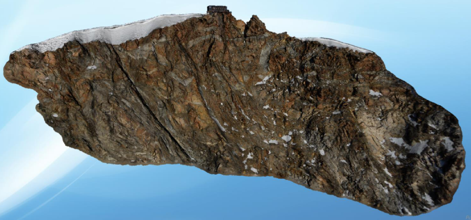
A thorough survey allowed describing the geomechanical features of Punta Gnifetti, by using laser scanner and photogrammetry, georadar and by performing direct measurements of the joint conditions. The reconstructed 3D model of the summit covers an area of some 200x100 m on the main rock face (Figure 2).

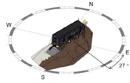
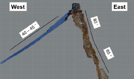
The summit is characterized by a main ridge, which runs approximately along the N-S direction, and two very different slopes on either side of it (Figure 1c). The west side has a moderate slope (40°/45°) and it is covered by a few metre thick layer of snow and ice. The east face (the dip direction is actually 117°) is characterized by a sub-vertical upper part, and a lower part with an inclination of approximately 65°.

The rock mass under the hut is mainly composed of paragneiss, and it is characterized by the presence of eight sets of joints (Table 1). The data obtained during the survey and the comparison with literature allowed evaluating the cohesion and friction angle of intact rock (c_r = 30 Mpa; Φ_r = 40°), as described in [5] and [8]. It is worth noting that, at the moment, no information is available regarding the presence of ice in depth. Therefore, both conditions of empty joints and ice filled joints have been considered in the simulations. Although the survey allowed evaluating the trace length for all joints sets, the correlation between this parameter and joint persistence is unreliable. Therefore, persistence will be determined during the back-analysis, as it will be described in the following.

Table 1. Geometry of joint sets.

Joint set	Dip direction (°)	Dip (°)	Spacing (m)
A	99	85	4.1
B	43	76	7.4
C	172	82	8.1
D	309	56	10.8
E	160	48	3.4
F	139	81	4.7
G	77	53	2.9
H	120	62	1.4

2. Numerical simulations

The numerical simulations are performed with the Distinct Element 3DEC code. Considering the low stress level, and for the sake of simplicity, rock blocks and the ice cover are modeled as rigid elements. Therefore the only model parameters are joint stiffness (almost irrelevant in a stability analysis) and resistance (see §2.2).

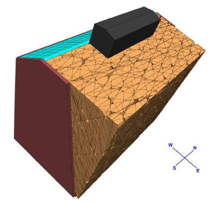
The numerical simulations are conducted by following the procedure suggested by Calvetti et al. [9], where an initial model with simplified geometry, but complete from the point of view of rock mass structure, is used (Figure 2). In this case the model is a 50x60x36 m (height x width x depth) parallelepiped. The hut is represented by a rigid element, and the back of the slope is cut to reproduce the geometry of the west flank and the presence of the ice cover.

Staring from this model, a back-analysis is performed first, where joint resistance is progressively decreased until the actual configuration of the slope is well reproduced (see §3). Starting from this point, joint resistance is further reduced to simulate evolutionary scenarios under various triggering conditions (see §4). A number of numerical simulations were preliminary performed with the aim of assessing the influence of the joint generation procedure and of boundary conditions [8]. These analyses are not shown here for the sake of brevity.

2.1. DEM model of the rock mass

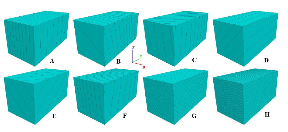
The joint sets introduced in the model (Figure 3) are directly based on the data of Table 1. It is worth noting that four sets are sub-vertical. Two of them are nearly parallel to the slope face (A and F) while the other two are almost perpendicular to it (B and C). Three joint sets with inclination between 50° and 60° form a sort of fan whose average dip direction is parallel to that of the slope (E, H and G). The remaining set dips in the opposite direction (D). In order to avoid unrealistically regular generation, the orientation of each joint is randomly picked within a ± 2° range from the values of Table1.

2.1. DEM model of the rock mass

The joint sets introduced in the model (Figure 3) are directly based on the data of Table 1. It is worth noting that four sets are sub-vertical. Two of them are nearly parallel to the slope face (A and F) while the other two are almost perpendicular to it (B and C). Three joint sets with inclination between 50° and 60° form a sort of fan whose average dip direction is parallel to that of the slope (E, H and G). The remaining set dips in the opposite direction (D). In order to avoid unrealistically regular generation, the orientation of each joint is randomly picked within a ± 2° range from the values of Table1.

2.2. Joint resistance and joint properties

Following the outcome of previous research [5], the Mohr-Coulomb criterion is here used for describing the resistance of discontinuous rock joints. In particular, in order to define the resistance parameters, in the simulations we adopt the formulae reported by Boffelli [8] - who elaborated the results by Wang ([5], [7]) - to describe the influence of persistence, k, on cohesion (c) and friction angle (Φ):

(1)

(2)

(3)

(4)

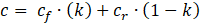
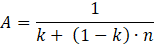
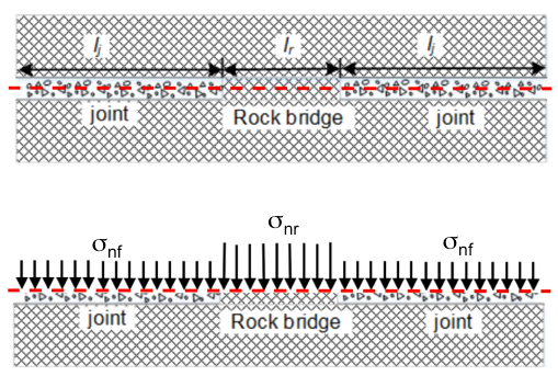
Where c_f and c_r are the cohesion of fill material and rock bridge, Φ_f and Φ_r are the friction angle of fill material and rock bridge, n is a stress concentration factor, σ _nf and σ _nr are the normal stress in the fill material and in the rock bridge (Figure 4).

(5)

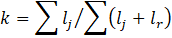
Where l_j and l_r are the length of cracked joint and of rock bridge (Figure 4).

It is worth noting that Eq. (2) represents an extension of the formula proposed by Jennings [10], who assumed that the normal stress is evenly distributed within the rock bridge and the fill material (i.e. n = 1). This is generally not the case as it is schematically shown in Figure 4: for example, values of n between 10 and 15 are reported in [5] for ice-filled joints on the basis of joint-scale DEM simulations. In the simulations shown in the following, n = 10 was assumed for ice filled joints. It is worth noting that Eq. (1) is the same formula proposed by Jennings [10], as its validity has been confirmed during previous research at the joint scale ([5], [7]). The joint tensile resistance is assumed to be half of the cohesion; furthermore, a fragile behaviour is assumed for the cohesive and tensile components [3].

Two conditions are analysed in the numerical simulations: empty joints (no fill material) and ice filled joints. It is worth to note that joint resistance reduces when the persistence increases (rock bridge fracturing) and/or temperature increases (which reduces the resistance of ice). These two driving factors will be separately considered in the following. As to the influence of temperature on the resistance of ice, on the basis of several (and often conflicting) literature correlations ([11]-[14]) the values of Table 2 are retained, as in [8].

Table 2. Ice strength parameters.

T (°C)	ci (kPa)	Φi (°)
-1	250	0
-2	500	0
-3	750	4
-4	1000	8

It is worth noting that the resistance of rock is much higher than that of ice (c_r = 30 Mpa; Φ_r = 40°, see §1.1). However, the contribution of ice cannot be neglected because of the very large k values that characterise the rock mass, as it will be shown in the following.

3. Back-analysis

Starting from the simplified model of Figure 3, a back-analysis procedure is performed by progressively reducing the joint resistance until the actual configuration of the slope is reproduced [9]. Back-analysis is performed under the two aforementioned conditions: empty joints and ice-filled joints. In this phase, a constant temperature is assumed, and the driving factor for strength reduction is considered to be the increase of persistence; strength parameters are calculated accordingly from Eqs. (1)-(2) and Table 2. In the case of ice-filled joints, the back-analysis has to be performed by assuming a value of temperature, first. Four values in the range from -4 to -1 °C have been considered in the simulations. For the sake of simplicity and as a preliminary check of the viability of the approach, at the moment a unique value of persistence and temperature is considered as representative of all the joint sets. This assumption is certainly simplistic, in that temperature is affected by depth and persistence may be different across the joint sets and be affected by the position of each individual joint.

3.1. Empty joints

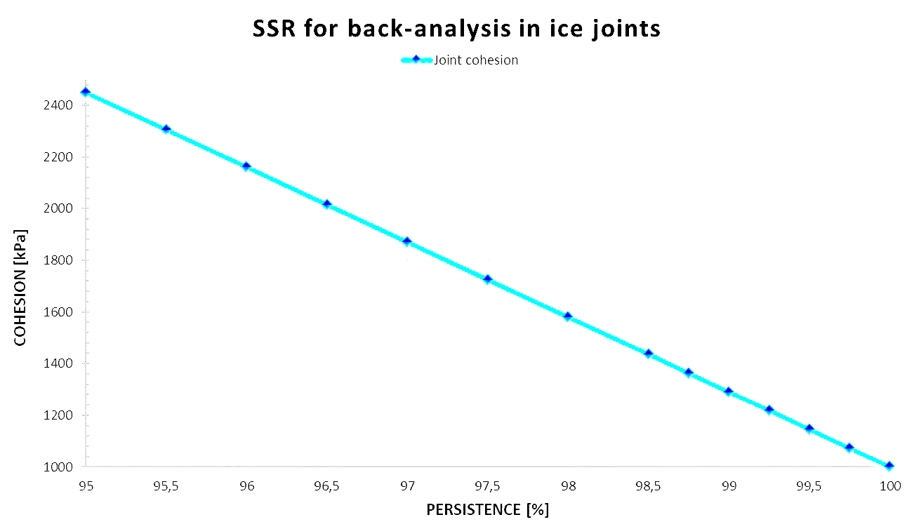
According to Eqs. (1)-(2), in the case of empty joints the increase of persistence involves a progressive reduction of joint cohesion; in particular, joint cohesion is proportional to the rock bridge relative extension, b = (1-k). On the contrary the joint friction angle is unaffected (note that n = ∞ in this case).

The results of numerical simulations clearly show that the increase in persistence corresponds to a progressive retrogression of the edge of the slope and to the reduction of the height of the sub-vertical portion of the profile (Figure 5).

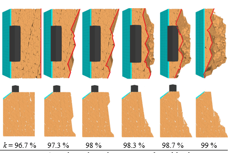
By analysing these results and comparing them with the actual slope profile, the realistic value of persistence can be easily selected (see §3.3). It is important to note that all configurations shown in Figure 5 (and in similar Figures in the following) represent stable states that are attained after each strength reduction step that is triggered by the increase in persistence. During each step, the unstable blocks are removed from the model.

3.2. Ice filled joints

According to Eqs. (1)-(2) and Table 2, the increase of persistence involves a progressive reduction of both joint cohesion and friction angle, with the trend being influenced by temperature. As an example, in Figure 6 the parameters corresponding to T = -4 °C are shown.

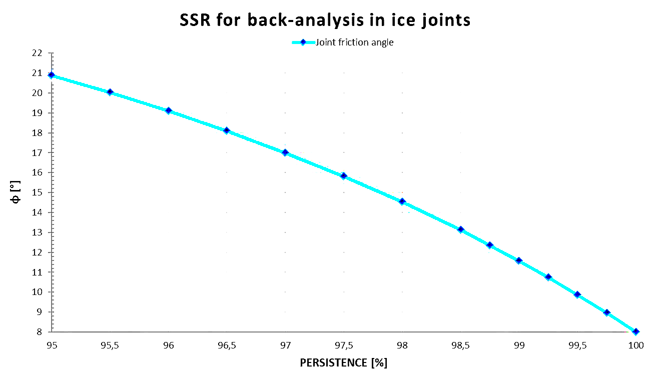
In Figure 7 the results obtained for T = -3 °C are taken as reference case. Similar results are obtained for the other temperature values considered in the simulation program.

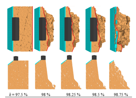
At first sight, the observed trend is similar to that obtained for empty joints (Figure 5). However, the retrogression of the slope is less progressive than in the previous case and it is characterised by a few big steps. By comparing the stable configurations of Figure 7 with the actual slope profile, the realistic value of persistence can be easily selected (see §3.3).

3.3. Discussion of results

The slope configurations that best reproduce the real slope are reported in Figure 8 for all the considered conditions. The values of persistence and relative rock bridge extension obtained from the back-analysis, and the corresponding strength joint parameters are reported in Table 3.

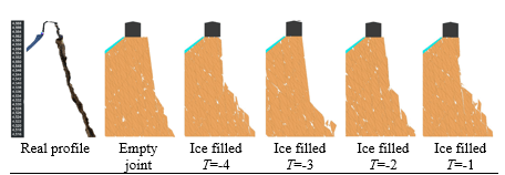
Table 3: Joint parameters calibrated from back-analysis (indicated with ₀ subscript).

Joint	T (°C)	k0 (%)	b0 = 1- k0 (%)	c0 (kPa)	Φ0 (°)
Empty	-	98.3	1.67	500	40
Ice filled	-1	96.5	3.5	1291	12.6
Ice filled	-2	97	3	1385	11.2
Ice filled	-3	98	2	1335	11.3
Ice filled	-4	98.75	1.25	1363	12.4

It is worth noting that in all cases it is possible to reproduce the actual slope profile with reasonable accuracy. The calibrated values of persistence are in general very large, i.e. close to 100%. The largest values of persistence correspond to the empty joint and to the lowest temperature for ice filled joints. This is consistent with the fact that for empty joints the friction angle is not affected by persistence and that the resistance contribution from ice larger at lower temperatures both in terms of friction and cohesion. It is worth noting that the empty joint condition is characterised by a “high friction/low cohesion” combination; the opposite combination occurs for the ice filled joints, with minor adjustments due to temperature variations. This difference is expected to influence the possible evolution of the rock slope that will be analysed in the following.

3.4. Reliability of results

It is important to note that results are affected by the initial configuration of the slope. In fact, as specified in §2.1, the generation of joints is characterised by the random choice of orientation within a ± 2° range. Therefore, and as consequence of the order of generation of joint sets, apparently slightly different configurations are obtained, as shown in Figure 9.

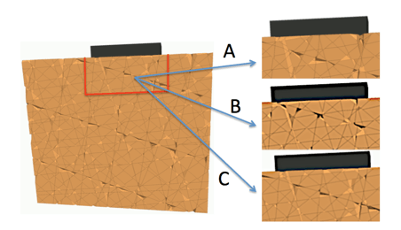
In order to assess the effect of joint generation it is useful to consider the effect of the SSR procedure on the evolution of the slope profile, which can be conveniently represented by the distance of the edge of the slope from the hut (Figure 10). Three models, which differ in the joint generation order, are considered here. Sub-vertical joints are generated first in model A; joints with dip orientation parallel and opposite to the dip orientation of the rock face are generated first in models B and C, respectively.

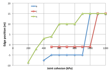
The results show that model A is characterised by a progressive evolution (retrogression) of the slope edge position. On the contrary, both with model B and C the evolution is much more irregular, as it is characterised by wide (in terms of cohesion range) stable phases and sudden large failures. This latter behaviour doesn’t seem to be realistic; therefore, all numerical simulations reported in this paper are performed with model A.

4. Scenarios of rock slope evolution

Starting from the reconstruction of the current configuration of Punta Gnifetti and the corresponding values of persistence and resistance parameters (Table 3), a strength reduction procedure can be applied in order to evaluate the margin of safety with respect to the future evolution of the slope.

In a traditional shear strength reduction method (SSR), resistance parameters are reduced by applying a factor R> 1, until a loss of stability occurs. The value of R at failure can then be interpreted as an overall factor of safety, F_s. In our case, a slightly different approach is followed where the reduction in resistance is directly associated with its triggering factor.

For empty joints, the triggering factor is identified with the progression of rock bridge damage, i.e. a further increase in persistence (or decrease in rock bridge extension). For ice filled joints, the considered triggering factor is temperature increase.

Obviously, in all cases the strength parameters at failure can be compared to the calibrated ones and an overall factor of safety, F_s, could be calculated. However, this value is just the outcome of the relationship among the set of factors that determine shear resistance of joints (i.e. persistence and temperature) and the mechanical behaviour. The assessment of the involved risk should include the evaluation of the probability that that a given value of persistence or temperature is actually attained.

4.1. Empty joints: fracture propagation

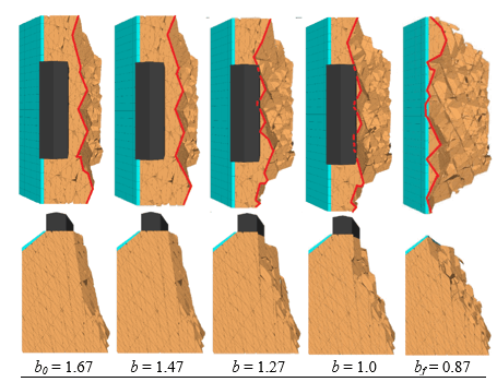
In this case, the resistance is progressively reduced by progressively increasing the persistence, i.e. reducing the rock bridge extension and joint cohesion.

According to Eqs. (1)-(2) this corresponds to a progressive reduction of cohesion, while friction angle is unaffected.

The corresponding evolution of the slope is shown in Figure 9. All in all, the trend is similar to that described in §3.1. In particular, a relatively regular retrogression of the edge of the slope is observed, until the configuration corresponding to the complete collapse of the peak is attained. This occurs for a value of relative rock bridge extension b_f ≈ b₀/2. In traditional terms, this would correspond to an overall factor of safety F_s ≈ 2; however, the interpretation of this result is not a direct indication of the associated risk, as previously discussed.

4.2. Ice filled joints: temperature increase

In this case, according to Table 3 and Eqs. (1)-(2), both cohesion and friction angle are gradually reduced as a consequence of increasing temperature. Note that in these simulations we have made the simplifying assumption that persistence is constant. This means that crack propagation is not considered among the consequences of stress redistribution, unless a complete failure of the bridge occurs.

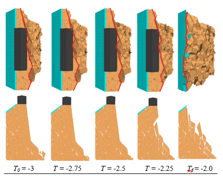
The evolution of the slope configuration is shown in Figure 10 for T0 = -3°. Similar results are obtained for the other investigated initial temperature values.

The results are characterized by a stable initial phase, followed by a sudden failure. This trend is similar to what observed during the back-analysis (see §3.2) and is qualitative different to the one that characterises the empty joint case.

This conclusion, that is valid both for back-analysis and the assessment of future scenarios, is probably associated with the fact that for ice filled joints the contribution of the cohesive term to overall resistance is larger (see Table 3), and that the cohesive term is fragile as previously reported. Under these conditions, it is expected that in the empty joint case slope retrogression is much more progressive than in the case of empty joints.

5. Conclusion

The results presented in this paper represent the application to a real case of the multi-scale approach proposed by the Authors; information from the material scale and joint scale ([5]-[7]) is here used to calculate the resistance of joints in a large scale DEM model. Given the lack of complete information about site conditions, a series of analyses are conducted under different hypotheses regarding joint conditions and temperature. For this reason, the presented results are to be considered indicative and more about the applicability of the approach than the reliable assessment of the stability conditions of the investigated site.

Despite current shortcomings and lack of information, the results of the simulations show that the numerical model can reproduce the current configuration of the considered rock face. In addition, the model was used to study the possible evolution of the rock slope, and in particular the instability that would arise in case of resistance degradation. In this respect, two external triggering factors, which are considered to be responsible of most real-world collapses, were simulated: the increase of joint persistence (which can be caused by repeated cycles of freeze/thaw); the increase in temperature. In both cases, the effects on the slope stability have been analysed and the trend of the evolution has been detected and qualitatively discussed. As a general comment, the obtained results indicate that rock bridges have a critical influence on the stability and evolution of rock slope, in particular due to the fact that persistence is close to 100%.

In order to improve the reliability of the numerical simulations, in situ investigation has to be integrated so that the actual conditions of the rock mass in depth are determined. The main points to be verified are the fracturing conditions in depth, the possible presence of ice and/or water, and the temperature profile with its fluctuations (daily, seasonal) and long term drift due to climate change.

Acknowledgements

The Authors acknowledge the financial and logistic support from Italian Alpine Club (CAI), and Imageo for the fundamental contribution to the geomechanical characterisation of the rock mass.

References

[1] M. Krautblatter, "Detection and quantification or permafrost change in alpine rock walls and implication for rock instability"y, Ph. D. Thesis, Universität Bonn, Germany, 2003.
[2] C. Harris, L.U. Arenson, H.H. Christiansen, B. Etzelmüller, R. Frauenfelder, S. Gruber, W. Haeberli, C. Hauck, M. Hölzle, O. Humlum, K. Isaksen, A. Kääb, M.A. Kern-Lütschg, M. Lehning, N. Matsuoka, J.B. Murton, J. Nötzli, M. Phillips, N. Ross, M. Seppälä, S.M. Springman and D. Vonder Mühll, "Permafrost and climate in Europe: Monitoring and modelling thermal, geomorphological and geotechnical responses. Earth Science Reviews, vol. 92, no. 3-4, pp. 117-171, 2009.
View Article
[3] M. Curtaz, A.M. Ferrero, R. Roncella, A. Segalini and G. Umili, "Terrestrial photogrammetry and numerical modelling for the stability analysis of rock slopes in high mountain areas: Aiguilles marbrées case", Rock mechanics and rock engineering, vol. 47, no. 2, pp. 605-620, 2014.
[4] M. Krautblatter, D. Funk and F. Günzel, "Why permafrost rocks become unstable: a rock-ice-mechanical model in time and space", Earth Surface Processes and Landforms, vol. 38, no. 8, pp. 876-887, 2013.
[5] G. Wang, "Modelling of permafrost degradation and gravity-induced risks in alpine areas," Ph.D. dissertation, Department ABC, Politecnico di Milano, Italy, 2022.
[6] G. Wang and F. Calvetti, "3D DEM investigation of the resistance of ice and frozen granular soils," European Journal of Environmental and Civil Engineering, vol. 26, no. 16, pp. 8242-8262, 2022.
[7] G. Wang and F. Calvetti, "DEM Modelling of Ice Filled Rock Joints," in Proceedings of the 16th International Conference IACMAG, Torino, Italy, 2021, pp. 941-948.
[8] W. Boffelli, "Numerical modelling of global warming effects on the stability of rock faces in high alps," M.Sc. dissertation, Civil Eng. For Risk Mitigation, Politecnico di Milano, Italy, 2022.
[9] F. Calvetti, T. Frenez, M. Vecchiotti, G. Piffer, V. Mair and D. Mosna, "DEM Simulation of the Evolution of an Unstable Rock Face: A Modelling Procedure for Back Analysis of Rockslides," Rock Mechanics and Rock Engineering, vol. 52, no. 1, pp. 149-161, 2019.
[10] J. Jennings, "A mathematical theory for the calculation of the stability of open cast mines," in Proceedings of Symp. on the Theoretical Background to the Planning of Open Pits, 1970, pp. 87-102.
[11] M.C. Davies, O. Hamza, B.W. Lumsden and C. Harris, "Laboratory measurement of the shear strength of ice-filled rock joints," Annals of Glaciology, vol. 31, pp. 463-467, 2000.
[12] P. Nater, L. Arenson and S. Springman, "Choosing geotechnical parameters for slope stability assessments in alpine permafrost soils," in Proceedings of the 9th International Conference on Permafrost, Fairbanks, AK, 2008, pp. 1261-1266.
[13] H.Y. Xu, Y.M. Lai, W.B. Yu, X.T. Xu and X.X. Chang, "Experimental research on triaxial strength of polycrystalline ice," Journal of Glaciology and Geocryology, vol. 33, no. 5, pp. 1120-1126, 2011.
[14] P. Mamot, S. Weber, T. Schröder and M. Krautblatter, "A temperature and stress controlled failure criterion for ice-filled permafrost rock joints," The Cryosphere, vol. 12, pp. 3333-3353, 2018.
[2] C. Harris, L.U. Arenson, H.H. Christiansen, B. Etzelmüller, R. Frauenfelder, S. Gruber, W. Haeberli, C. Hauck, M. Hölzle, O. Humlum, K. Isaksen, A. Kääb, M.A. Kern-Lütschg, M. Lehning, N. Matsuoka, J.B. Murton, J. Nötzli, M. Phillips, N. Ross, M. Seppälä, S.M. Springman and D. Vonder Mühll, "Permafrost and climate in Europe: Monitoring and modelling thermal, geomorphological and geotechnical responses. Earth Science Reviews, vol. 92, no. 3-4, pp. 117-171, 2009. View Article
[3] M. Curtaz, A.M. Ferrero, R. Roncella, A. Segalini and G. Umili, "Terrestrial photogrammetry and numerical modelling for the stability analysis of rock slopes in high mountain areas: Aiguilles marbrées case", Rock mechanics and rock engineering, vol. 47, no. 2, pp. 605-620, 2014. View Article
[4] M. Krautblatter, D. Funk and F. Günzel, "Why permafrost rocks become unstable: a rock-ice-mechanical model in time and space", Earth Surface Processes and Landforms, vol. 38, no. 8, pp. 876-887, 2013. View Article
[6] G. Wang and F. Calvetti, "3D DEM investigation of the resistance of ice and frozen granular soils," European Journal of Environmental and Civil Engineering, vol. 26, no. 16, pp. 8242-8262, 2022. View Article
[7] G. Wang and F. Calvetti, "DEM Modelling of Ice Filled Rock Joints," in Proceedings of the 16th International Conference IACMAG, Torino, Italy, 2021, pp. 941-948. View Article
[9] F. Calvetti, T. Frenez, M. Vecchiotti, G. Piffer, V. Mair and D. Mosna, "DEM Simulation of the Evolution of an Unstable Rock Face: A Modelling Procedure for Back Analysis of Rockslides," Rock Mechanics and Rock Engineering, vol. 52, no. 1, pp. 149-161, 2019. View Article
[11] M.C. Davies, O. Hamza, B.W. Lumsden and C. Harris, "Laboratory measurement of the shear strength of ice-filled rock joints," Annals of Glaciology, vol. 31, pp. 463-467, 2000. View Article
[14] P. Mamot, S. Weber, T. Schröder and M. Krautblatter, "A temperature and stress controlled failure criterion for ice-filled permafrost rock joints," The Cryosphere, vol. 12, pp. 3333-3353, 2018. View Article