1. Introduction

The design of tailings dams involves the necessity to perform nonlinear dynamic analyses (NDAs) to verify the seismic stability of the dams, especially in areas of high seismicity such as the South American Andes, which are part of the Pacific Ring of Fire. On a large scale, the tectonic framework is determined by the interaction between the Nazca and South American plates. In the current state of practice for seismic evaluation of slope displacements in subduction tectonic settings, several procedures are available (e.g., [1,2]). These available procedures can be used to estimate permanent displacements in tailings dams, with certain limitations. However, when potentially liquefiable materials affect the seismic performance of structures, more rigorous procedures, such as nonlinear dynamic analyses, should be employed.

Fragility curves are one of the key elements of probabilistic seismic risk assessment of the built environment and lifeline system [3]. They relate the IMs to the probability of reaching or exceeding a damage state (e.g., minor, moderate, major, severe, collapse) for each element at risk. Given the diversity of ground motion IMs, several researchers have evaluated their effectiveness, predictability, and total uncertainty. Recently, studies have been conducted on the uncertainty analysis of different IMs in predicting damage levels. Regina et al. [4], found that the CAV is the optimal IM in predicting the vulnerability of earth dams and the fragility functions based on the CAV have the lowest standard deviation values. Armstrong et al. [5], found that the AI was the most efficient IM, however, the CAV has the lower total standard deviation in the evaluation of earth dams. Boada et al. [6] propose fragility curves for abandoned tailings dams in Chile as a function of the spectral acceleration at a vibration period of 0.3s, Sa(0.3s), this IM shows a lower efficiency but was finally selected due to its high predictability when compared to the more efficient alternatives.

The purpose of this study is to present fragility functions and efficiency analyses of IMs to assess the probability of damage levels for a tailings dam based on horizontal crest displacements. Furthermore, according to the results, it would be possible to define alert levels to be considered in the operation manual of the tailings storage facility (TSF) and design criteria.

2. Numerical modelling

The tailings dam geometry considered in this study is representative of an existing Peruvian tailings dam constructed using the downstream method (referent to rockfill). The numerical modelling is performed using the commercial 2D finite difference software platform FLAC [7], which is based on an explicit time-marching method to solve the equations of motion. The zone sizes in FLAC are chosen to ensure accurate high frequencies wave transmission based on the recommendations of Kuhlemeyer and Lysmer [8]. Ground motion frequencies greater than 15 Hz were filtered out, as they carry a relatively small amount of energy, as described by Mánica et al [9]. The size of the FLAC zones was 1.0 m in both vertical and horizontal directions. In the model, the boundaries were sufficiently far from the failure zone to minimize the influence of the boundaries on the model response. A free field boundary condition was applied to the side boundaries and a quiet boundary was considered at the bottom boundary in both the horizontal and vertical directions during the dynamic analyses.

The outcrop input motions were applied in a form of shear stress at the base of the model using the compliant-base procedure of Mejia and Dawson [10]. A Rayleigh damping of 0.5% at a centre frequency of 2.5 Hz was used during the dynamic loading. The tailings were assumed to be saturated and liquefiable; therefore, the fourth columns of the zones at the far left boundary was assumed to be non-liquefiable to avoid inaccurate free field boundary calculations, as recommended by Boulanger and Ziotopoulou [11]. The initial stress state for the tailings dam is estimated using a five-state procedure. Seepage analyses are performed with an uncoupled fluid flow calculation, groundwater boundary conditions were applied to the model to obtain a water table that descends through the filter/drain location and to ensure a saturated condition for the tailings.

Three different constitutive models are used in this study. For the materials susceptible to liquefaction (tailings), the PM4Silt V2.1 model [11] is used. The behaviour of the foundation bedrock is assumed to be linear elastic, while all the other materials are characterized by the UBCHyst model [12]. PM4Silt is a plane strain-stress ratio-controlled, critical state-compatible, bounding surface plasticity model for clays and plastic silts and has recently been used to represent tailings (e.g., [13,14,15]). Calibration of this model is performed with single-element simulations for the range of loading paths important for the tailings. In this study, the PM4Silt parameters are calibrated to obtain a cyclic resistance to liquefaction curve that matches that estimated from cyclic direct simple shear (CDSS) tests. UBCHyst is a robust, relatively simple, total stress model. It uses the Mohr-Coulomb failure criterion, extended with a formulation for shear secant modulus reduction with strain. The UBCHyst parameters of the rockfill and filter/drain material are calibrated to be consistent with the G/G_max ratio and damping curves of Rollins et al. [16] and Darendeli [17], respectively. The filter/drain material is located between the rockfill-tailings and rockfill-bedrock interfaces.

Figure 1 shows the dam geometry model generated in FLAC. The bedrock has a length of 1100 m and a thickness of 50 m, the tailings have a height of 100 m, and the rockfill has a height of 101 m with a crest length of 10 m. The downstream slope is a 2.0H:1.0V and the upstream slope is 1.5H:1.0V.

The rockfill strength parameters for the dynamic analyses were estimated based on average data from Leps [18]. The friction angle ϕ' was estimated based on Barton and Kjaersnli [19], using Eq. 1.

(1)

Where σ'3, ϕ1, Δϕ and Pa are minor principal effective stress, reference friction angle (at σ'₃=Pa), friction angle reduction for each log cycle of stress level increase, and atmospheric pressure, respectively.

In the case of the filter/drain and rockfill, G_max was estimated using the Eq. 2 proposed by Seed et al. [20]. The bedrock was simulated as an elastic material with a stiffness corresponding to shear wave velocity of 760 m/s and the stiffness properties of the tailings were obtained from the resonant column and torsional shear (RCTS) test calibrated with the parameters considered for the PM4Silt model.

(2)

Where G_max, k_2,max, and p' are the small strain shear modulus, modulus coefficient, and the mean effective pressure, respectively.

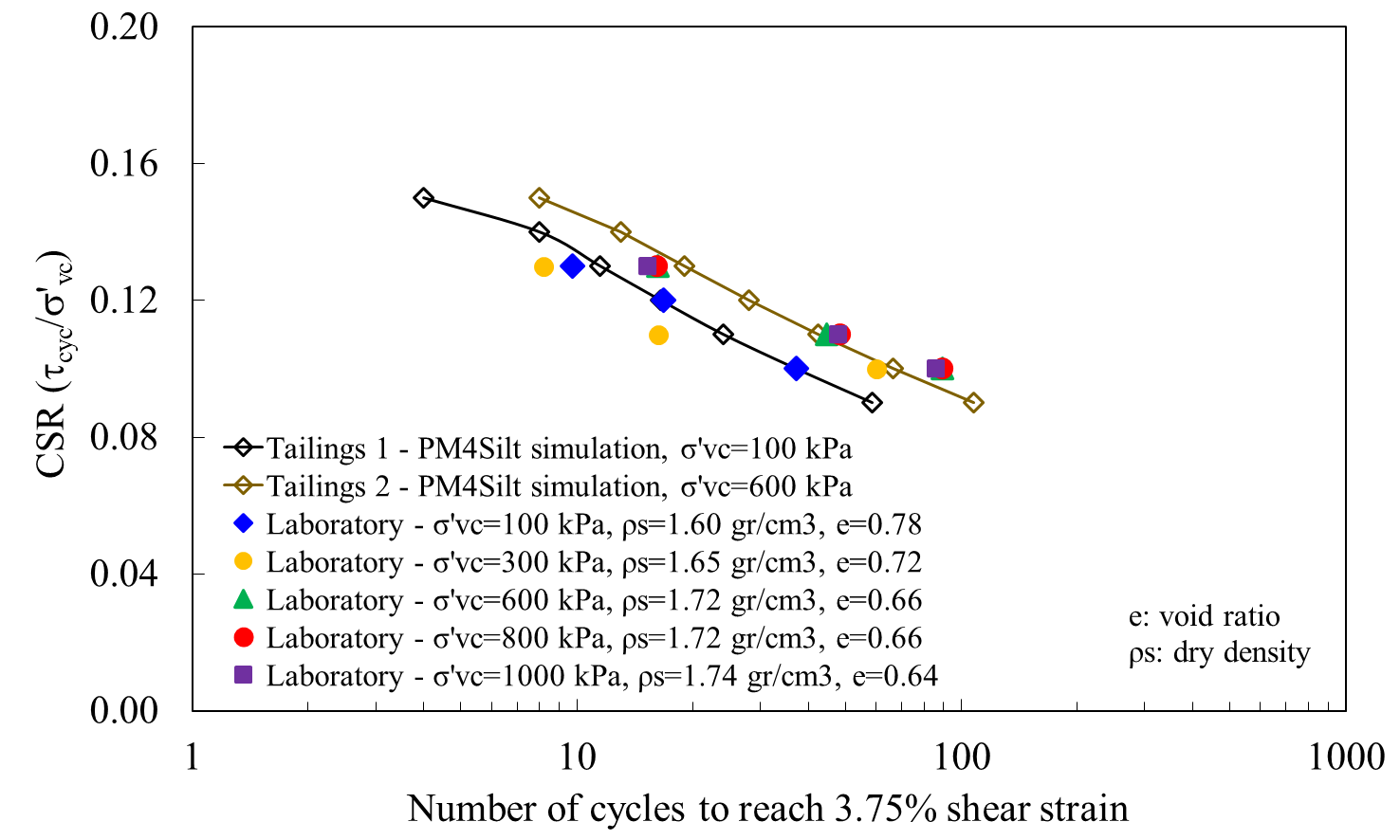
The summary of the parameters in the dynamic analysis for a tailings dam is shown in Table 1. Tailings parameters are shown in Table 1 (the secondary parameters for the PM4Silt model not shown in the table were kept at the default value) divided by an effective vertical stress (σ'_vc) of 400 kPa (according to laboratory test, see Figure 2). Tailings 1, σ'_vc ≤ 400 kPa and Tailings 2, σ'_vc > 400 kPa.

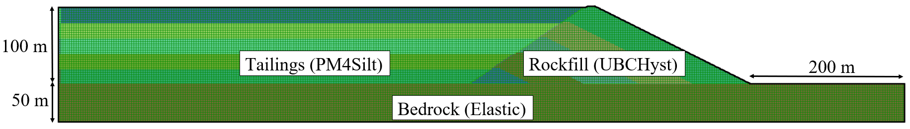
Table 1. Parameters adopted for the dynamic analysis for a tailings dam.

Input parameters	Rockfill	Filter/drain	Tailings 1/2	Bedrock
Dry unit weight, γdry (kN/m3)	22	16	16.3 / 17.5	25
Cohesion, c'	-	0	-	-
Friction angle, ϕ'	ϕ1=45.5, Δϕ=6.55	35	-	-
Small strain shear modulus, Gmax (MPa)	-	-	-	1500
Modulus coefficient, k2,max	180	110	-	-
Poisson ratio, ʋ	0.30	0.33	-	0.25
PM4Silt
Undrained shear strength ratio at critical state, Su,cs/σ'vc	-	-	0.15 / 0.15	-
Shear modulus coefficient, Go	-	-	602 / 602	-
Contraction rate parameter, hpo	-	-	5.5 / 10	-
Initial void ratio, eo	-	-	0.8 / 0.66	-
Shear modulus exponent, nG	-	-	0.7 / 0.7	-
Critical state friction angle, ϕ'cv	-	-	31 / 31	-
Compressibility in e-ln(p') space, λ	-	-	0.06 / 0.06	-
Sets bounding pmin, ru,max	-	-	0.98 / 0.98	-
UBCHyst
Hn	1	1	-	-
Hrf	0.7	0.98	-	-
Hrm	1	1	-	-
Hdfac	0.8	0.6	-	-
Hdmodf1	2	1	-	-

Cycle simple shear tests were performed to investigate the cyclic response and liquefaction resistance curves of the tailings. The sample was sheared under a harmonic sinusoidal loading at 0.05 Hz, with amplitude characterized by a defined cyclic stress ratio (CSR is the ratio of the cyclic shear stress to the initial vertical effective stress).

Figure 2 shows the derived PM4Silt based cyclic resistance curves calibration against laboratory cyclic direct simple shear (CDSS) for a cyclic strain of 3.75%. In concordance with Macedo et al. [13], the slopes of the liquefaction resistance curves for tailings are flatter than typical curves for sands and do not present an important sensitivity in terms of the confinement stress before the cyclic loading.

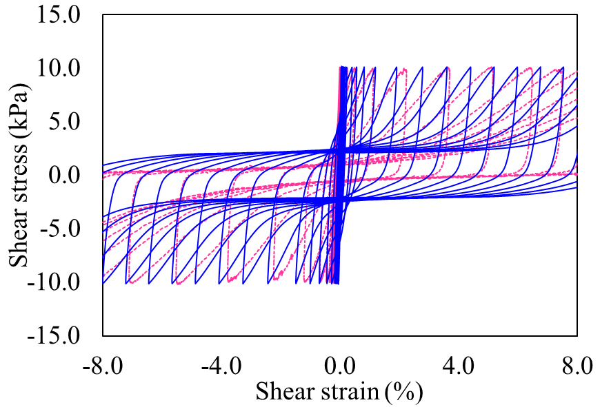
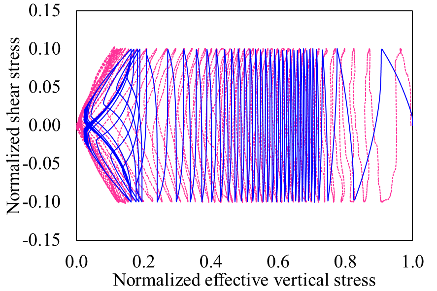
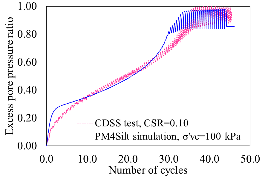
Figure 3 shows the ability of the PM4Silt model to capture the undrained cyclic behaviour of the tailings, successfully capturing the key cyclic behaviour in terms of cyclic strain accumulation and pore pressure generation.

(a)	(b)
(c)	(d)

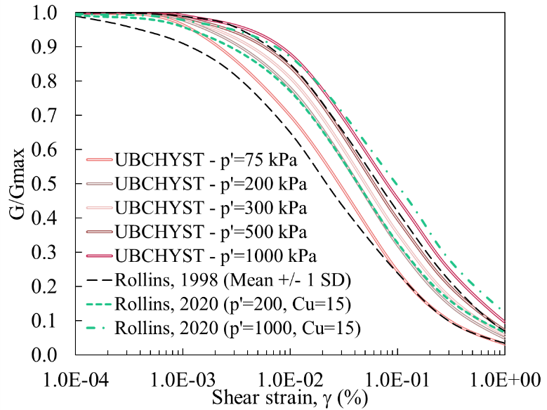
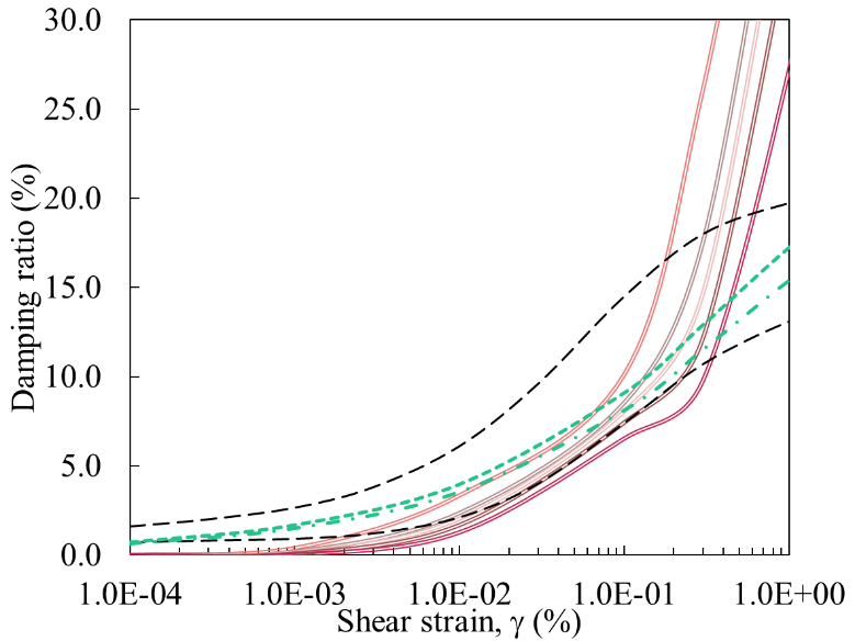
Figure 4 shows a comparison of the G/G_max and damping ratio curves calibrated in FLAC for the rockfill with the curves from Rollins et al. [16].

The UBCHYST model follows an extended Masing rule; hence, it tends to overestimate the experiment-based hysteretic damping curves at large strain (e.g., Figure 4). Macedo et al. [13], recommend that future studies should explore the implementation and performance of non-Masing models in NDAs of TSFs.

(a)

(b)

3. Input ground motions

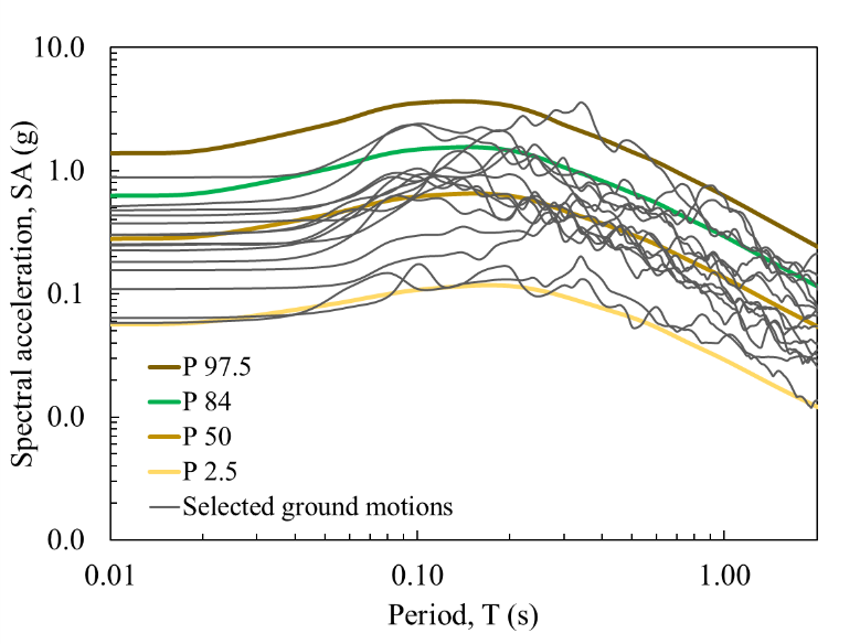
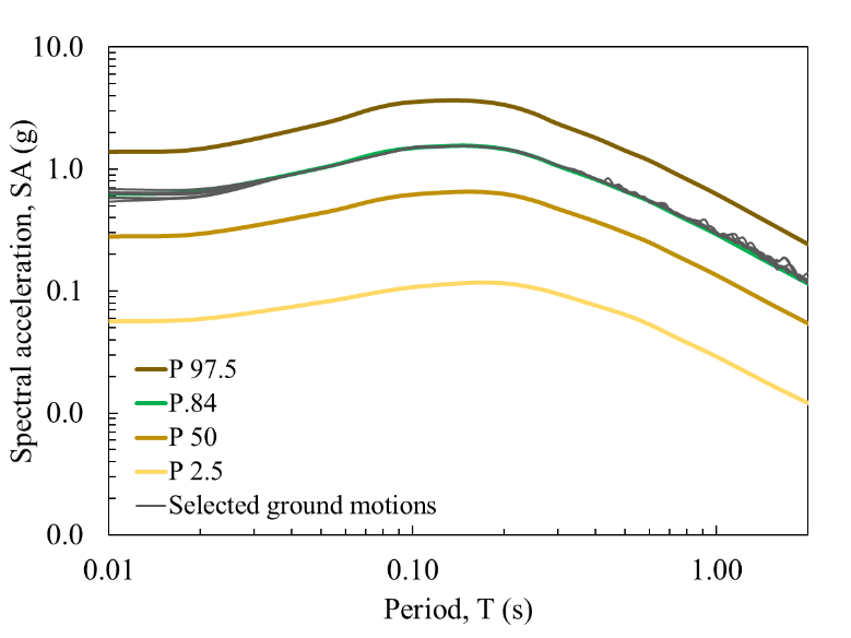
Two methods were considered for the selection of ground motions. The first one, described by Baker and Lee [21], for which candidate ground motions were selected from different institutions such as CISMID, CSN, IGP, COSMOS, and RENADIC. The generated database contains more than 251 ground motions, mainly from interface and intraslab subduction earthquakes recorded in Chile and Peru. According to this methodology, a total of 15 ground motions (with an average shear wave velocity in the upper 30 m, between 600 m/s≤V_s30≤950 m/s) were selected, that were compatible with the Maximum Credible Earthquake (MCE 50th percentile) and its associated standard deviation obtained from the deterministic seismic hazard analysis (DSHA) for soil type BC (ASCE 7-22), V_s30=760 m/s. The second method involves the generation of ground motions using the spectral matching method (described by Al Atik and Abrahamson [22]), 7 ground motions were considered with a target spectrum obtained from the 84th percentile MCE, these ground motions correspond to intraslab earthquakes.

The first method was considered to include ground motions with different intensity measures that are collectively compatible with a target spectrum and its associated standard deviation. Meanwhile, the second method, which is commonly used in current engineering practice, provides ground motions that are compatible with a target spectrum without having variability in the response spectra; however, they have different intensity measures. Figure 5 shows the response spectra of the 22 selected ground motions compared to the response spectra of the MCE with different percentiles.

4. Evaluation of optimal ground motion intensity measures

According to Regina et al. [4], the correlation between an intensity measure (IM) and the target damage measure (DM) can be synthesized by a single property of the selected IM: its efficiency (i.e., how well the IM is correlates with a given DM). The estimated IMs of the input ground motions for this study were peak ground acceleration PGA, peak ground velocity PGV, Arias intensity AI, and spectral accelerations SA. Rathje and He [23], described that the median of the structural demand in terms of IM (note that SD is the model prediction of DM), can be expressed in Eq. 3:

(3)

It is also assumed that the DM model follows a lognormal distribution. Thus, the distribution of the logarithm of the data (e.g., ln(DM)) at a given IM follows a normal distribution with a mean given by Eq. 3 and a standard deviation of σlnDM|lnIM. This standard deviation of the regression model in Eq. 3, using the predicted and the measured values, is given by Eq. 4:

(4)

where DM_i is the recorded maximum value of the demand parameter from each analysis and N is the number of analyses performed.

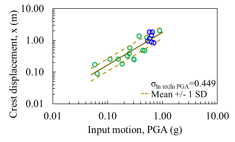
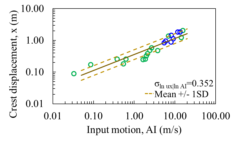
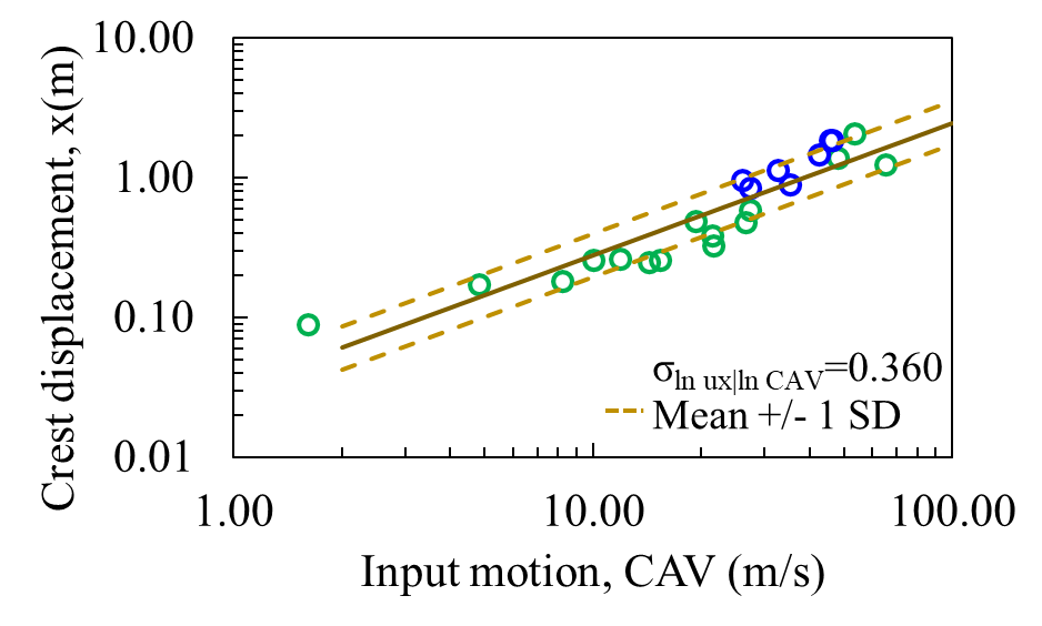
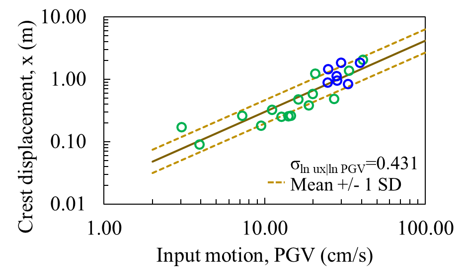
In the present study, we considered the horizontal crest displacement as a DM. However, different DMs could be considered, such as: filter displacement, free board reduction, normalized crest settlement and even the excess pore water pressure (r_u) for materials that pose a risk to the seismic stability of TSFs. Figure 6 shows the horizontal crest displacements with some intensity measures (PGA, AI, CAV, and PVG) of the input ground motions. The green circles show the input ground motions from the methodology developed by Baker and Lee [21], and the blue circles show those obtained by the spectral matching methodology.

Analysis of IM predictability is incorporated as suggested by Armstrong et al. [5] by calculating the total standard deviation as Eq. 5:

(5)

where σ_lnIM|M,R,S is the standard deviation of a ground motion model (GMM), representing its predictability, and b is the slope of the least-square linear regression on a log-log scale.

However, for the present evaluation, the standard deviations representing the predictability, were estimated by the conditional ground motion models (CGMMs, σ_{lnIMsec|lnIMp}), according to the 84th percentile MCE, for different IMs such as AI, CAV, and PGV developed by Macedo et al [24] and Liu and Macedo [25,26], respectively. These CGMMs were developed for subduction earthquakes. Finally, the analysis of the optimal IM considering CGMMs is as follows Eq. 6:

(5)

where IM_sec represents a secondary IM and IM_p represents the observed primary IM, as described by Macedo et al. [27]. Table 2 shows the efficiency, predictability, and total standard deviation for AI, CAV, and PGV. IM_CGMMs represents the intensity measure estimated by the CGMMs (units: AI m/s, CAV m/s, PGV cm/s).

Table 2. Efficiency, predictability, and total standard deviation for horizontal crest displacements.

IM	Efficiency σlnDM|lnIMsec	Predictability σlnIMsec|lnIMp	Total SD σlnDM|lnIMp	IMCGMMs
AI	0.352	0.331	0.389	7.59
CAV	0.360	0.302	0.459	31.57
PGV	0.431	0.374	0.603	24.23

(a)

(b)

The horizontal displacements at the crest obtained at the end of the seismic action were evaluated based on the intensity measures of input ground motions (see Figure 6). It is observed that the Arias Intensity has the lower dispersion (standard deviation) in estimating the displacements.

The results obtained from the ground motions spectrally matched to the MCE P.84 demonstrate significant variability in terms of displacements, indicating that the selection of design earthquakes is not a trivial procedure. The CGMMs can be used to select the design earthquake with an intensity measure given earthquake scenario and site conditions.

(a)	(b)
(c)	(d)

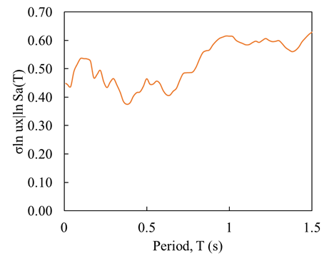
The efficiency of the 5% damped spectral acceleration at different periods Sa(T) is quantified through the dispersion σ_lnDM|lnIM in Figure 7a. In the figure, the dispersion decreases for periods close to the fundamental vibration period of the dam, T=0.4 s (undamped analysis, estimate in FLAC). This range of high efficiency (i.e., low dispersion σ_lnDM|lnIM) may be associated with the resonance of the dam and stiffness degradation that occurs in the model.

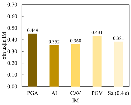
Figure 7b summarizes the efficiencies of the five tested IMs: Peak Ground Acceleration (PGA), Arias Intensity (AI), Cumulative Absolute Velocity (CAV), and Spectral Acceleration at 0.4 s [Sa(0.4 s)]. Figure 7b indicates that AI is the most efficient IM for estimating Ux in this model. Furthermore, the spectral acceleration at a period of 0.4 s shows a high efficiency than other spectral accelerations.

(a)

(b)

5. Fragility functions for different IMs

The seismic performance of tailings dams can be evaluated using fragility functions, which provide the probability of structures reaching (or exceeding) a given limit state (or damage measure, DM) for each level of ground motion intensity measure (IM). It can be expressed as Eq. 7:

(7)

In this study, analytical fragility functions are considered because they are based on the results of numerical models. A lognormal cumulative distribution function (CDF) is often used to define a fragility function [3] (see, Eq. 8).

(8)

where Φ is the standard normal CDF, x is the IM, θ is the IM corresponding to 50% exceedance probability (i.e., the median), and β is the total natural log standard deviation.

The development of the fragility curves according to Eq. 8 requires the estimation of θ and β from the results of dynamic analyses. Following the approach of HAZUS [28], the uncertainty associated with the definition of the damage measure states (β_DS) is set equal to 0.4. The uncertainty associated with the capacity (β_C) is set equal to 0.25. The last source of uncertainty, related to the seismic demand, is described by the variability of the response due to the variability of the ground motions (β_D= σ_lnDM|lnIM, efficiency). β is defined as Eq. 9.

(9)

Baker [29] presents various methods for computing fragility functions for structural systems (e.g., incremental dynamic analysis, IDA; multiple stripe analysis, MSA), which have recently been used by different researchers (e.g., [4,6]) to evaluate dams because they use a significant number of earthquakes. However, in the present evaluation, the 22 earthquakes described above, which are compatible with the MCE spectrum, were considered for the construction of fragility curves according to the procedure of Argyroudis et al. [3].

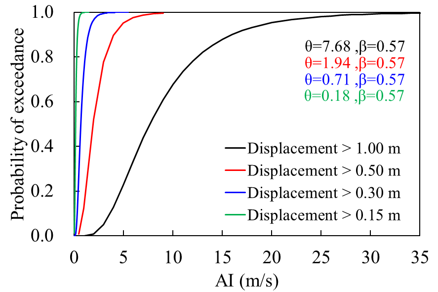
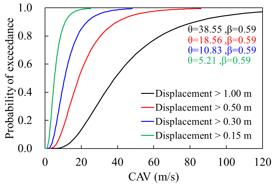
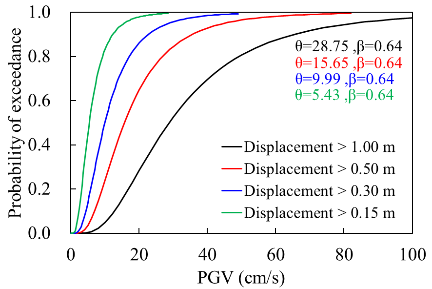
Figure 8 shows the fragility functions for the horizontal crest displacements as DM with some values of the limiting displacement (i.e., 1.00, 0.50, 0.25, and 0.15 m). In the Figure 8b, considering the mean Arias Intensity estimated by CGMM (see Table 2, AI: 7.59 m/s), a probability of exceedance of 100% is obtained for displacements greater than 0.50 m, while a 40% probability for displacements greater than 1.0 m. It is necessary to consider the dispersion in the estimation of the AI (e.g., according CGMMs) or other IMs as well as the uncertainty parameters in the generation of the fragility functions (β) to estimate a range of exceedance probability of design.

(a)	(b)
(c)	(d)

5. Conclusion

This study presents the seismic performance of a tailings dam in central Peru, located in an area of high seismicity. The geotechnical characterization was used to provide inputs to the PM4Silt model, which was used to represent the cyclic response of the tailings and the UBCHyst model was used for the rockfill and filter/drain, as they are not expected to generate pore pressure under cyclic loading.

The correlation between IMs and DM (horizontal displacements) for the tailings dam indicated that the most efficient and optimal IM was the AI in predicting the horizontal crest displacements and it is found that the spectral acceleration at a period of 0.4s (fundamental period of the tailings dam), Sa (0.4s), shows a high efficiency than other spectral accelerations.

The available fragility functions for the tailings dam vulnerability assessment could be used to define alert levels under seismic loading with a certain level of risk that is acceptable for a tailings dam. CGMMs are developed to estimate IMs (e.g., AI, CAV, PGV) for earthquakes in subduction zones that have a lower total standard deviation than those estimated by traditional GMMs. These estimated IMs are consistent with a given spectral acceleration of the design response spectrum (e.g., 84th percentile MCE). The IMs estimated by CGMMs, along with the fragility curves, can be used to define a range of exceedance probability of design.

In current engineering practice, the spectral matching methodology is commonly employed to generate design earthquakes. From the results obtained from the spectral matching of seven earthquakes, a dispersion of results is observed, highlighting the importance of considering a wide range of seismic records for the evaluation of seismic performance of geotechnical structures.

References

[1] J. D. Bray, J. Macedo, and T. Travasarou, "Simplified Procedure for Estimating Seismic Slope Displacements for Subduction Zone Earthquakes," Journal of Geotechnical and Geoenvironmental Engineering, vol. 144, no. 3, Mar. 2018, doi: 10.1061/(ASCE)GT.1943-5606.0001833.
View Article
[2] J. Macedo, J. D. Bray, and C. Liu, "Seismic Slope Displacement Procedure for Interface and Intraslab Subduction Zone Earthquakes," Journal of Geotechnical and Geoenvironmental Engineering, vol. 149, no. 11, Nov. 2023, doi: 10.1061/JGGEFK.GTENG-11445.
[3] S. Argyroudis, A. M. Kaynia, and K. Pitilakis, "Development of fragility functions for geotechnical constructions: Application to cantilever retaining walls," Soil Dynamics and Earthquake Engineering, vol. 50, pp. 106-116, Jul. 2013, doi: 10.1016/j.soildyn.2013.02.014.
[4] G. Regina, P. Zimmaro, K. Ziotopoulou, and R. Cairo, "Evaluation of the optimal ground motion intensity measure in the prediction of the seismic vulnerability of earth dams," Earthquake Spectra, vol. 39, no. 4, pp. 2352-2378, Nov. 2023, doi: 10.1177/87552930231170894.
[5] R. Armstrong, T. Kishida, and D. Park, "Efficiency of ground motion intensity measures with earthquake-induced earth dam deformations," Earthquake Spectra, vol. 37, no. 1, pp. 5-25, Feb. 2021, doi: 10.1177/8755293020938811.
[6] G. Boada, C. Pasten, and P. Heresi, "Analytical fragility curves for abandoned tailings dams in North-Central Chile," Soil Dynamics and Earthquake Engineering, vol. 164, p. 107637, Jan. 2023, doi: 10.1016/j.soildyn.2022.107637.
[7] Inc. (2019) Itasca Consulting Group, "FLAC - Fast Lagrangian Analysis of Continua, Ver. 8.1." Minneapolis: Itasca.
[8] R. L. Kuhlemeyer and J. Lysmer, "Finite Element Method Accuracy for Wave Propagation Problems," Journal of the Soil Mechanics and Foundations Division, vol. 99, no. 5, pp. 421-427, May 1973, doi: 10.1061/JSFEAQ.0001885.
[9] M. Mánica, E. Ovando, and E. Botero, "Assessment of damping models in FLAC," Comput Geotech, vol. 59, pp. 12-20, Jun. 2014, doi: 10.1016/j.compgeo.2014.02.007.
[10] L. Mejia and E. Dawson, "Earthquake Deconvolution for FLAC," in Fourth International FLAC Symposium on Numerical Modeling in Geomechanics, Madrid, Spain, May 2006. [Online]. Available:
[11] R. W. Boulanger and K. Ziotopoulou, "PM4Silt (Version 2.1): A silt plasticity model for earthquake engineering applications," Center for Geotechnical Modeling, Department of Civil and Environmental Engineering, University of California, Davis, CA, Report No. UCD/CGM-23/02, Feb. 2023.
[12] E. Naesgaard, "A Hybrid Effective Stress-Total Stress Procedure for Analyzing Soil Embankments Subjected to Potential Liquefaction and Flow," Ph. D. dissertation, The University of British Columbia, Vancouver, BC, Canada, 2011.
[13] J. Macedo, P. Torres, L. Vergaray, S. Paihua, and C. Arnold, "Dynamic effective stress analysis of a centreline tailings dam under subduction earthquakes," Proceedings of the Institution of Civil Engineers - Geotechnical Engineering, vol. 175, no. 2, pp. 224-246, Apr. 2022, doi: 10.1680/jgeen.21.00017a.
[14] A. Cerna-Diaz, M. Kafash, R. Davidson, L. Yenne, and P. Doughty, "Nonlinear Deformation Analyses of a Tailings Dam during a Mw5.7 Earthquake," in Geo-Congress 2023, Reston, VA: American Society of Civil Engineers, Mar. 2023, pp. 70-85. doi: 10.1061/9780784484708.007.
[15] S. Salam, M. Xiao, A. Khosravifar, and K. Ziotopoulou, "Seismic stability of coal tailings dams with spatially variable and liquefiable coal tailings using pore pressure plasticity models," Comput Geotech, vol. 132, p. 104017, Apr. 2021, doi: 10.1016/j.compgeo.2021.104017.
[16] K. M. Rollins, M. Singh, and J. Roy, "Simplified Equations for Shear-Modulus Degradation and Damping of Gravels," Journal of Geotechnical and Geoenvironmental Engineering, vol. 146, no. 9, Sep. 2020, doi: 10.1061/(ASCE)GT.1943-5606.0002300.
[17] M. B. Darendeli, "Development of a New Family of Normalized Modulus Reduction and Material Damping Curves," Ph. D. dissertation, University of Texas, TX, USA, 2001.
[18] T. M. Leps, "Review of Shearing Strength of Rockfill," Journal of the Soil Mechanics and Foundations Division, vol. 96, no. 4, pp. 1159-1170, Jul. 1970, doi: 10.1061/JSFEAQ.0001433.
[19] N. Barton and B. Kjaersnli, "Shear strength of rockfill," International Journal of Rock Mechanics and Mining Sciences & Geomechanics Abstracts, vol. 18, no. 6, p. 111, Dec. 1981, doi: 10.1016/0148-9062(81)90543-X.
[20] H. B. Seed, R. T. Wong, I. M. Idriss, and K. Tokimatsu, "Moduli and Damping Factors for Dynamic Analyses of Cohesionless Soils," Journal of Geotechnical Engineering, vol. 112, no. 11, pp. 1016-1032, Nov. 1986, doi: 10.1061/(ASCE)0733-9410(1986)112:11(1016).
[21] J. W. Baker and C. Lee, "An Improved Algorithm for Selecting Ground Motions to Match a Conditional Spectrum," Journal of Earthquake Engineering, vol. 22, no. 4, pp. 708-723, Apr. 2018, doi: 10.1080/13632469.2016.1264334.
[22] L. Al Atik and N. Abrahamson, "An Improved Method for Nonstationary Spectral Matching," Earthquake Spectra, vol. 26, no. 3, pp. 601-617, Aug. 2010, doi: 10.1193/1.3459159.
[23] E. M. Rathje and J. He, "A Seismic Fragility Framework for Earth Dams," in Lifelines 2022, Reston, VA: American Society of Civil Engineers, Nov. 2022, pp. 405-415. doi: 10.1061/9780784484432.036.
[24] J. Macedo, N. Abrahamson, and J. D. Bray, "Arias intensity conditional scaling ground-motion models for subduction zones," Bulletin of the Seismological Society of America, vol. 109, no. 4, pp. 1343-1357, Aug. 2019, doi: 10.1785/0120180297.
[25] C. Liu and J. Macedo, "New conditional, scenario-based, and non-conditional cumulative absolute velocity models for subduction tectonic settings," Earthquake Spectra, vol. 38, no. 1, pp. 615-647, Feb. 2022, doi: 10.1177/87552930211043897.
[26] C. Liu and J. Macedo, "New conditional, scenario-based, and traditional peak ground velocity models for interface and intraslab subduction zone earthquakes," Earthquake Spectra, vol. 38, no. 3, pp. 2109-2134, Aug. 2022, doi: 10.1177/87552930211067817.
[27] J. Macedo, C. Liu, and N. A. Abrahamson, "On the Interpretation of Conditional Ground-Motion Models," Bulletin of the Seismological Society of America, vol. 112, no. 5, pp. 2580-2586, Oct. 2022, doi: 10.1785/0120220006.
[28] Federal Emergency Management Agency, "Hazus Earthquake Model Technical Manual - Hazus 5.1," 2022.
[29] J. W. Baker, "Efficient Analytical Fragility Function Fitting Using Dynamic Structural Analysis," Earthquake Spectra, vol. 31, no. 1, pp. 579-599, Feb. 2015, doi: 10.1193/021113EQS025M.
[1] J. D. Bray, J. Macedo, and T. Travasarou, "Simplified Procedure for Estimating Seismic Slope Displacements for Subduction Zone Earthquakes," Journal of Geotechnical and Geoenvironmental Engineering, vol. 144, no. 3, Mar. 2018, doi: 10.1061/(ASCE)GT.1943-5606.0001833. View Article
[2] J. Macedo, J. D. Bray, and C. Liu, "Seismic Slope Displacement Procedure for Interface and Intraslab Subduction Zone Earthquakes," Journal of Geotechnical and Geoenvironmental Engineering, vol. 149, no. 11, Nov. 2023, doi: 10.1061/JGGEFK.GTENG-11445. View Article
[3] S. Argyroudis, A. M. Kaynia, and K. Pitilakis, "Development of fragility functions for geotechnical constructions: Application to cantilever retaining walls," Soil Dynamics and Earthquake Engineering, vol. 50, pp. 106-116, Jul. 2013, doi: 10.1016/j.soildyn.2013.02.014. View Article
[4] G. Regina, P. Zimmaro, K. Ziotopoulou, and R. Cairo, "Evaluation of the optimal ground motion intensity measure in the prediction of the seismic vulnerability of earth dams," Earthquake Spectra, vol. 39, no. 4, pp. 2352-2378, Nov. 2023, doi: 10.1177/87552930231170894. View Article
[5] R. Armstrong, T. Kishida, and D. Park, "Efficiency of ground motion intensity measures with earthquake-induced earth dam deformations," Earthquake Spectra, vol. 37, no. 1, pp. 5-25, Feb. 2021, doi: 10.1177/8755293020938811. View Article
[6] G. Boada, C. Pasten, and P. Heresi, "Analytical fragility curves for abandoned tailings dams in North-Central Chile," Soil Dynamics and Earthquake Engineering, vol. 164, p. 107637, Jan. 2023, doi: 10.1016/j.soildyn.2022.107637. View Article
[8] R. L. Kuhlemeyer and J. Lysmer, "Finite Element Method Accuracy for Wave Propagation Problems," Journal of the Soil Mechanics and Foundations Division, vol. 99, no. 5, pp. 421-427, May 1973, doi: 10.1061/JSFEAQ.0001885. View Article
[9] M. Mánica, E. Ovando, and E. Botero, "Assessment of damping models in FLAC," Comput Geotech, vol. 59, pp. 12-20, Jun. 2014, doi: 10.1016/j.compgeo.2014.02.007. View Article
[10] L. Mejia and E. Dawson, "Earthquake Deconvolution for FLAC," in Fourth International FLAC Symposium on Numerical Modeling in Geomechanics, Madrid, Spain, May 2006. [Online]. Available: View Article
[13] J. Macedo, P. Torres, L. Vergaray, S. Paihua, and C. Arnold, "Dynamic effective stress analysis of a centreline tailings dam under subduction earthquakes," Proceedings of the Institution of Civil Engineers - Geotechnical Engineering, vol. 175, no. 2, pp. 224-246, Apr. 2022, doi: 10.1680/jgeen.21.00017a. View Article
[14] A. Cerna-Diaz, M. Kafash, R. Davidson, L. Yenne, and P. Doughty, "Nonlinear Deformation Analyses of a Tailings Dam during a Mw5.7 Earthquake," in Geo-Congress 2023, Reston, VA: American Society of Civil Engineers, Mar. 2023, pp. 70-85. doi: 10.1061/9780784484708.007. View Article
[15] S. Salam, M. Xiao, A. Khosravifar, and K. Ziotopoulou, "Seismic stability of coal tailings dams with spatially variable and liquefiable coal tailings using pore pressure plasticity models," Comput Geotech, vol. 132, p. 104017, Apr. 2021, doi: 10.1016/j.compgeo.2021.104017. View Article
[16] K. M. Rollins, M. Singh, and J. Roy, "Simplified Equations for Shear-Modulus Degradation and Damping of Gravels," Journal of Geotechnical and Geoenvironmental Engineering, vol. 146, no. 9, Sep. 2020, doi: 10.1061/(ASCE)GT.1943-5606.0002300. View Article
[18] T. M. Leps, "Review of Shearing Strength of Rockfill," Journal of the Soil Mechanics and Foundations Division, vol. 96, no. 4, pp. 1159-1170, Jul. 1970, doi: 10.1061/JSFEAQ.0001433. View Article
[19] N. Barton and B. Kjaersnli, "Shear strength of rockfill," International Journal of Rock Mechanics and Mining Sciences & Geomechanics Abstracts, vol. 18, no. 6, p. 111, Dec. 1981, doi: 10.1016/0148-9062(81)90543-X. View Article
[20] H. B. Seed, R. T. Wong, I. M. Idriss, and K. Tokimatsu, "Moduli and Damping Factors for Dynamic Analyses of Cohesionless Soils," Journal of Geotechnical Engineering, vol. 112, no. 11, pp. 1016-1032, Nov. 1986, doi: 10.1061/(ASCE)0733-9410(1986)112:11(1016). View Article
[21] J. W. Baker and C. Lee, "An Improved Algorithm for Selecting Ground Motions to Match a Conditional Spectrum," Journal of Earthquake Engineering, vol. 22, no. 4, pp. 708-723, Apr. 2018, doi: 10.1080/13632469.2016.1264334. View Article
[22] L. Al Atik and N. Abrahamson, "An Improved Method for Nonstationary Spectral Matching," Earthquake Spectra, vol. 26, no. 3, pp. 601-617, Aug. 2010, doi: 10.1193/1.3459159. View Article
[23] E. M. Rathje and J. He, "A Seismic Fragility Framework for Earth Dams," in Lifelines 2022, Reston, VA: American Society of Civil Engineers, Nov. 2022, pp. 405-415. doi: 10.1061/9780784484432.036. View Article
[24] J. Macedo, N. Abrahamson, and J. D. Bray, "Arias intensity conditional scaling ground-motion models for subduction zones," Bulletin of the Seismological Society of America, vol. 109, no. 4, pp. 1343-1357, Aug. 2019, doi: 10.1785/0120180297. View Article
[25] C. Liu and J. Macedo, "New conditional, scenario-based, and non-conditional cumulative absolute velocity models for subduction tectonic settings," Earthquake Spectra, vol. 38, no. 1, pp. 615-647, Feb. 2022, doi: 10.1177/87552930211043897. View Article
[26] C. Liu and J. Macedo, "New conditional, scenario-based, and traditional peak ground velocity models for interface and intraslab subduction zone earthquakes," Earthquake Spectra, vol. 38, no. 3, pp. 2109-2134, Aug. 2022, doi: 10.1177/87552930211067817. View Article
[27] J. Macedo, C. Liu, and N. A. Abrahamson, "On the Interpretation of Conditional Ground-Motion Models," Bulletin of the Seismological Society of America, vol. 112, no. 5, pp. 2580-2586, Oct. 2022, doi: 10.1785/0120220006. View Article
[29] J. W. Baker, "Efficient Analytical Fragility Function Fitting Using Dynamic Structural Analysis," Earthquake Spectra, vol. 31, no. 1, pp. 579-599, Feb. 2015, doi: 10.1193/021113EQS025M. View Article