1. Introduction

Multistage direct shear testing provides an efficient alternative to traditional singlestage tests for evaluating the shear strength of soils. This is particularly relevant for coarse-grained or mixed-grained soils, where the material demand and equipment requirements for large-scale testing can be substantial. In comparison to the conventional approach, which typically requires three independent tests on identical specimens, the multistage method reduces testing time and resource consumption [1]-[6]. However, accurate application of the multistage procedure requires careful control of each shear phase, especially in dense soils. Excessive mobilization during the early stages can lead to structural degradation within the shear zone, affecting the validity of the final results. Several studies have shown that terminating the first and second shear phases before reaching the peak strength is crucial to preserving key strength components such as structure, bonding, and dilatancy [1]-[6]. These components, only present in the initial stages, may not be recovered once disturbed, leading to underestimation of peak shear strength in subsequent stages [15]. Despite its advantages, the multistage test is often avoided due to the uncertainty in interpreting partially mobilized curves. To address this issue, the ability to estimate the peak shear strength before failure becomes essential. Predicting the shear behavior from incomplete curves allows for the design of more effective multistage testing procedures. This approach minimizes sample disturbance while maintaining the accuracy of shear strength estimation.

This study introduces a model that enables the prediction of peak shear strength and the corresponding shear displacement based on partially mobilized data from direct shear tests. The model is adapted from Kondner’s (1963) [7] hyperbolic function, traditionally applied to triaxial tests, and is fitted through normalization and regression techniques. The model is validated using a comprehensive dataset of 484 direct shear tests, performed on coarse-, fine-, and mixed-grained soils. The resulting framework provides a method to estimate peak values when early termination occurs, improving the interpretation of incomplete shear curves.

2. Background and Theoretical Model

The behavior of soils under shear loading can be effectively described using nonlinear stress–strain relationships. One of the most widely recognized formulations in this context is the hyperbolic function introduced by Kondner (1963) [7] to approximate the stress–strain curves of soils in drained triaxial tests. Duncan and Chang (1970) [8] later incorporated this concept into an elastoplastic constitutive model, which has since served as a foundation for various soil models, including the widely used Hardening Soil model.

In its original form, the hyperbolic model expresses the mobilization of deviator stress (q) as a function of axial strain (ε), governed by two key parameters, a and b, where a represents the inverse of the initial tangent modulus (E_i) at the beginning of the shearing phase, and b defines the asymptotic stress level. The basic hyperbolic formulation is expressed as:

(1)

Where q is the deviator stress, σ₁ and σ₃ are the principal stresses, ε represents the axial strain, and a and b are constants derived from regression analysis of experimental data. As axial strain increases, the deviator stress approaches an asymptotic limit q_a, defined by:

As axial strain increases, the deviator stress approaches an asymptotic limit q_a, defined by:

(2)

Where q_a is the asymptotic deviator stress, σ₁ and σ₃ are the principal stresses, and b is a constant as previously defined.

The asymptotic deviator stress (q_a) is related to the failure deviator stress (q_f) through the failure ratio R_f. A typical value for R_f is 0.9, but for most soils, it falls between 0.75 and 1.0 [10]. The relationship is expressed as:

(3)

Where q_f and (σ₁-σ₃)_f represent the failure deviator stress, and R_f is the failure ratio, which is less than or equal to 1.0.

By substituting the constant a in Eq. 1 with the inverse of the initial elastic modulus (E_i) and replacing b using the expressions from Eqs. 2 and 3, the following expression is obtained:

(4)

Where q is the deviator stress, σ₁ and σ₃ are the principal stresses, ε represents the axial strain, E_i represents the initial elastic modulus, (σ₁-σ₃)_f is the failure deviator stress, and R_f is the failure ratio.

This form enables the estimation of the stress–strain curve based on known material stiffness and failure parameters. The hyperbolic model's flexibility and simplicity have led to its widespread use for approximating stress paths up to failure in triaxial testing.

This formulation serves as the foundation for developing a predictive model applicable to direct shear tests.

3. Model Adaptation for Direct Shear Tests

Although the hyperbolic formulation was originally developed for triaxial conditions, its structure allows it to be adapted to other test configurations. In direct shear testing, the deviator stress (q) is replaced by a normalized shear stress (τ_norm), and the axial strain (ε) by a normalized horizontal shear displacement (s_h,norm). These normalized variables are obtained by dividing the shear stress and displacement values by the peak shear stress (τ_p) and the corresponding shear displacement (s_h,p ), respectively. The normalized variables are defined as follows:

(5)

Where τ_norm is the normalized shear stress, τ is the shear stress, and τ_p is the peak shear stress.

(6)

Where s_h,norm is the normalized horizontal shear displacement, s_h is the horizontal shear displacement, and s_h,p is the horizontal displacement at peak shear strength.

Substituting these into the hyperbolic model yields the following expression for normalized shear stress as a function of normalized shear displacement:

(7)

Where τ_norm is the normalized shear stress, s_h,norm is the normalized shear displacement, and a and b are dimensionless parameters obtained through regression based on the normalized data up to the peak.

This transformation reduces sensitivity to scale and allows for a more stable and reliable parameter estimation across tests with different stress levels or displacements.

Figure 1 presents the normalized shear stress–displacement curve fitted using the hyperbolic model (solid blue line). The inset graph shows the corresponding unnormalized curve, where the blue segment represents the data used for fitting (up to the peak shear strength), and the green segment shows the post-peak behavior. This representation highlights the normalization process and the portion of the data relevant for model calibration.

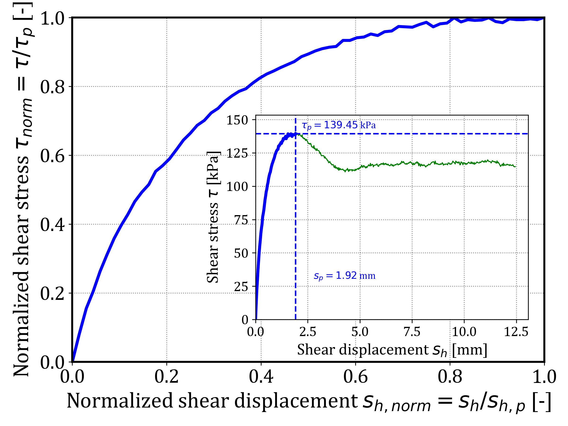
The use of normalized variables significantly improves the stability and reliability of the regression by reducing sensitivity to outliers and inconsistencies, particularly at low displacements. In addition, normalization ensures consistent axis scaling, which is especially important when applying nonlinear regression techniques such as the hyperbolic model.

4. Data and Materials

To evaluate the applicability of the normalized hyperbolic model to direct shear tests, an extensive dataset was compiled from experiments conducted between 2010 and 2023 at the Geotechnical Laboratory of the University of Applied Sciences in Dresden. The dataset includes 484 direct shear tests performed on 175 different soil types, representing a wide spectrum of grain sizes and mechanical behaviors.

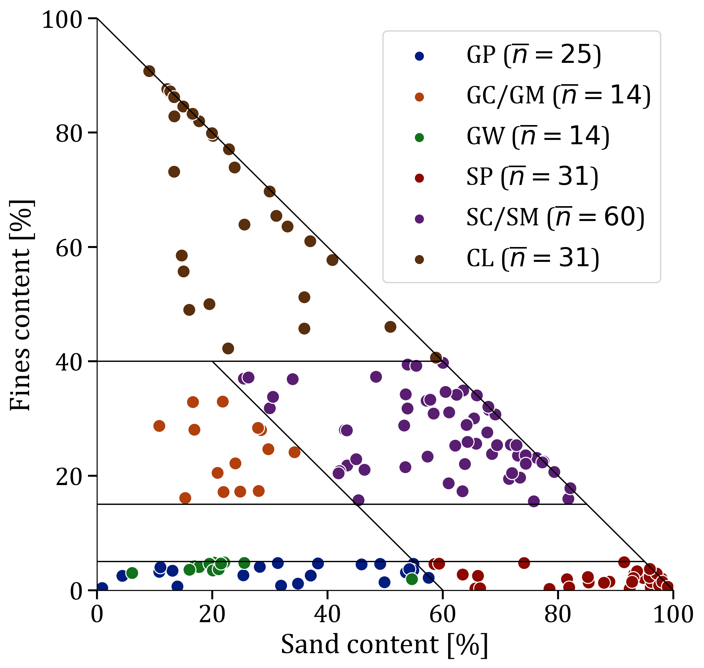
The soils were classified into six main groups according to the Unified Soil Classification System (USCS): GW (well-graded gravel), GP (poorly graded gravel), GC/GM (clayey and silty gravel), SP (poorly graded sand), SC/SM (clayey and silty sand), and CL (low-plasticity clay). Figure 2 shows the distribution of the 175 tested soils based on their fines and sand content, grouped by USCS classification. The number of tested soils per group is indicated in parentheses, highlighting the diversity of the materials analyzed within each classification.

Each test specimen was compacted to a relative density ranging from 88% to 100%. The initial water content varied between 1% and 54%, depending on the material type and compaction method.

Four different direct shear devices were used across the test program, each calibrated to ensure comparability of results.

The tests were conducted under drained conditions, and the applied normal stresses varied depending on the expected strength of each soil type. For model fitting, only the shear stress and horizontal displacement data were considered. Each curve was normalized as described in Section 3, and only the portion up to the peak shear strength was used, as shown in Figure 1.

4. 1. Validation and Model Fitting

The available data enabled the determination of the peak shear strength τ_p and the shear displacement at failure s_h,p. These values were used to normalize the shear stress–displacement curves according to Eqs. 5 and 6. The normalized data were then fitted using Eq. 7, with the parameters a and b determined through nonlinear regression. Given the known values of the constant b and the peak shear stress τ_p, the failure ratio R_f was calculated using Eqs. 2 and 3. The parameter R_f plays a central role in assessing the validity of the model, as its values should fall within the typical range reported in the literature. According to [9], typical R_f values for triaxial tests range from 0.5 to 1.0.

Figure 3 shows the distribution of R_f values obtained from all 484 tests. The data approximate a normal distribution with a mean of 0.791 and a standard deviation of 0.139.

The majority of the values fall within the expected range of 0.5 to 1.0, with only 4% of tests (20 shear tests) yielding R_f values between 0.3 and 0.5. These lower values were observed primarily in the GW and GP soil groups. Low R_f values are typically associated with dense or overconsolidated soils, whereas higher values tend to occur in loosely packed or normally consolidated soils.

Selected examples of fitted curves are presented in Figure 4. The orange and blue curves illustrate cases with lower coefficients of determination due to local fluctuations in the measurements, whereas the red and green curves show well-fitted data with high agreement between model and measurements.

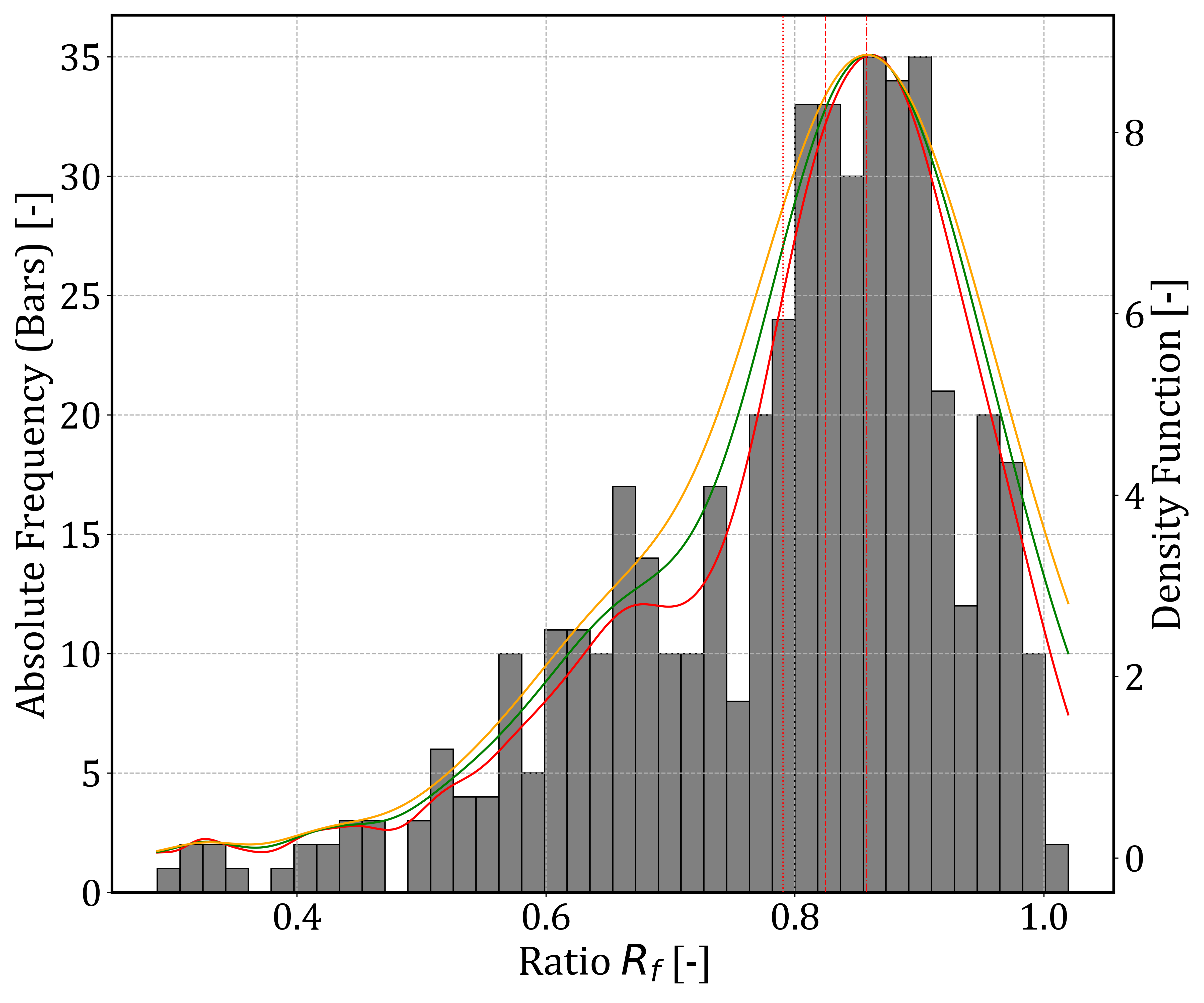
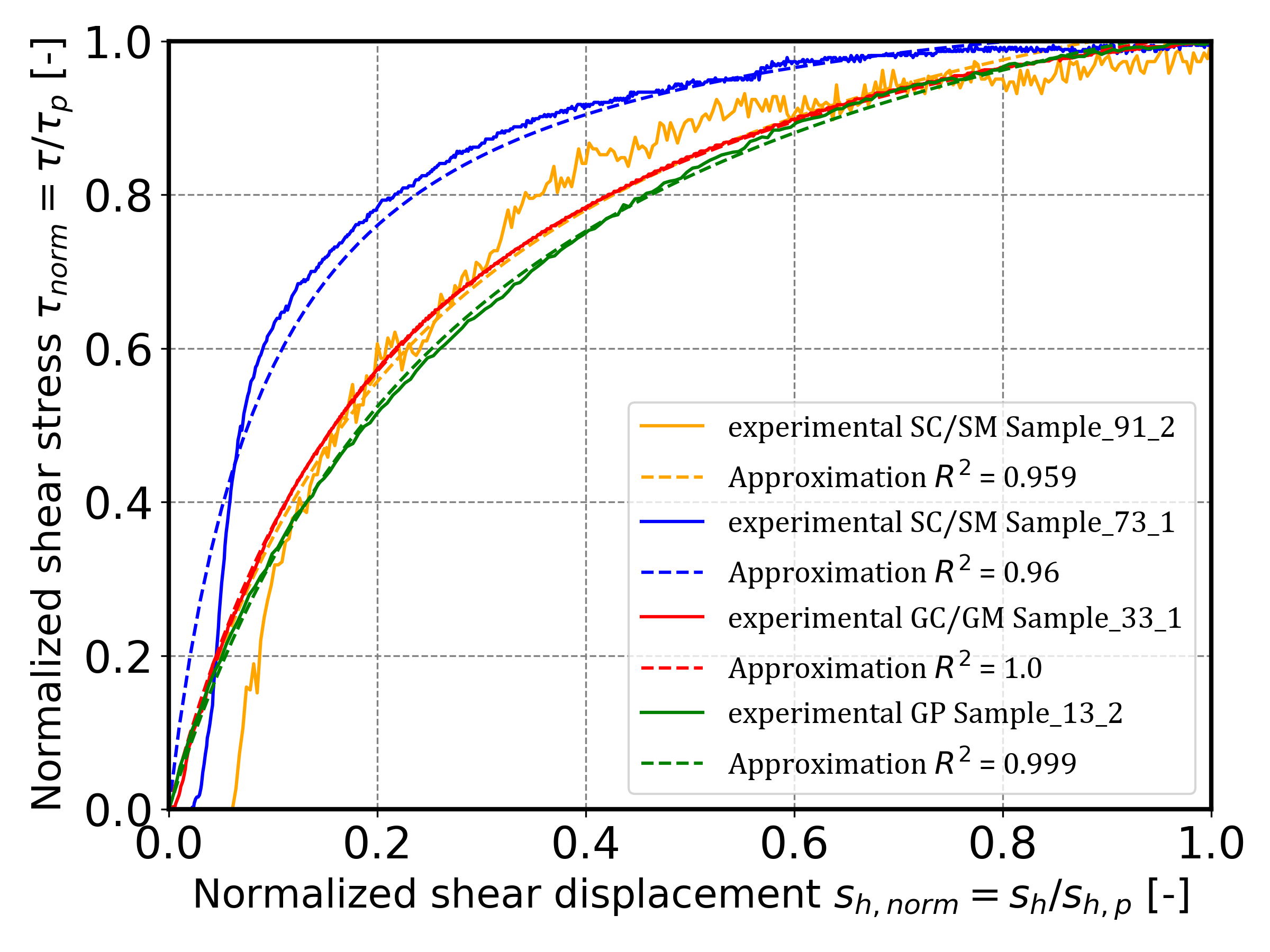
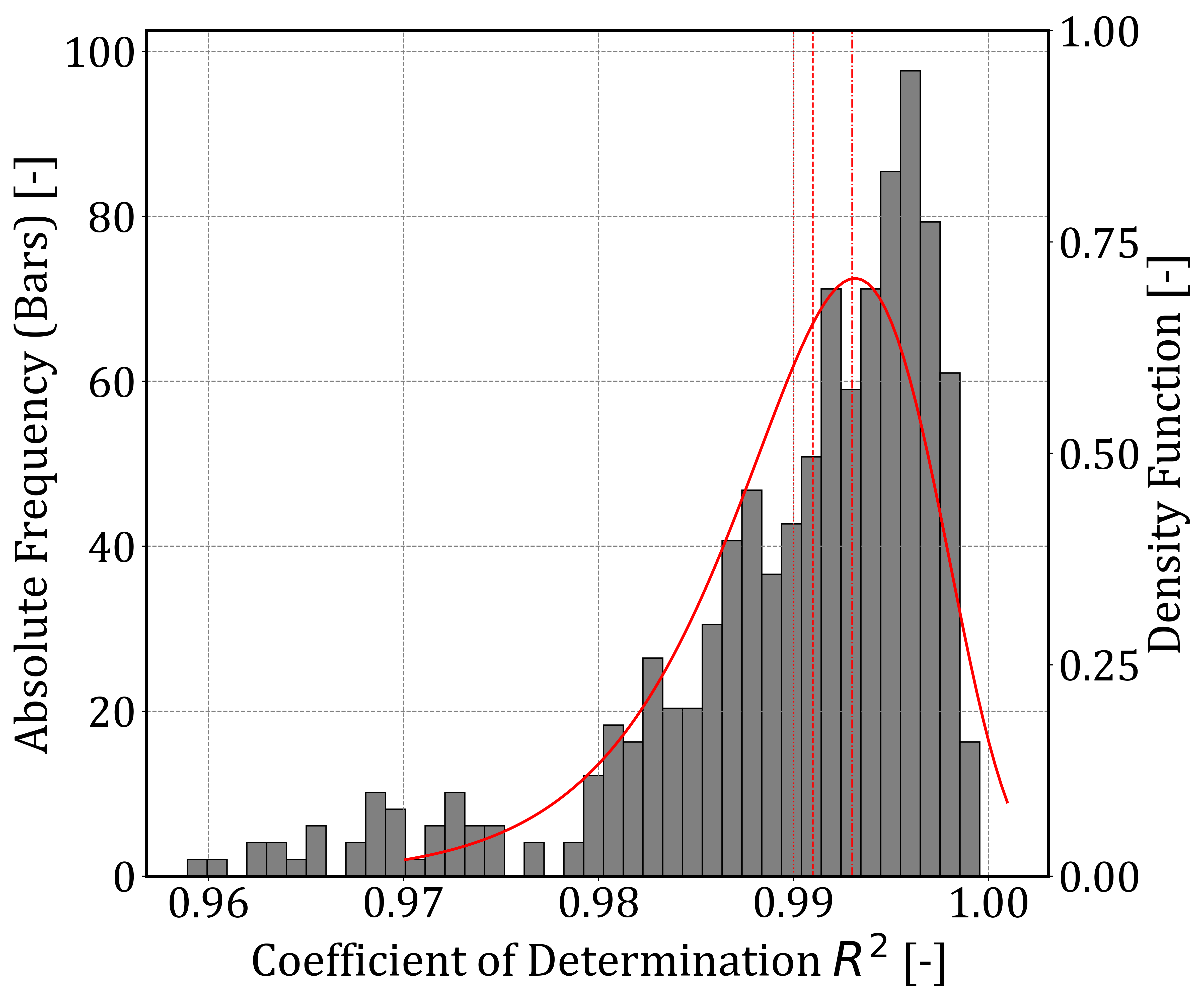
Figure 5 displays the distribution of all R² values obtained from the fitted models. The data follow a Weibull distribution with scale and shape parameters of 0.993 and 195.71, respectively. These results confirm that the normalized hyperbolic model provides a consistent and accurate fit across a wide range of soil types and test conditions.

4. 2. Interpretation of Parameters a and b

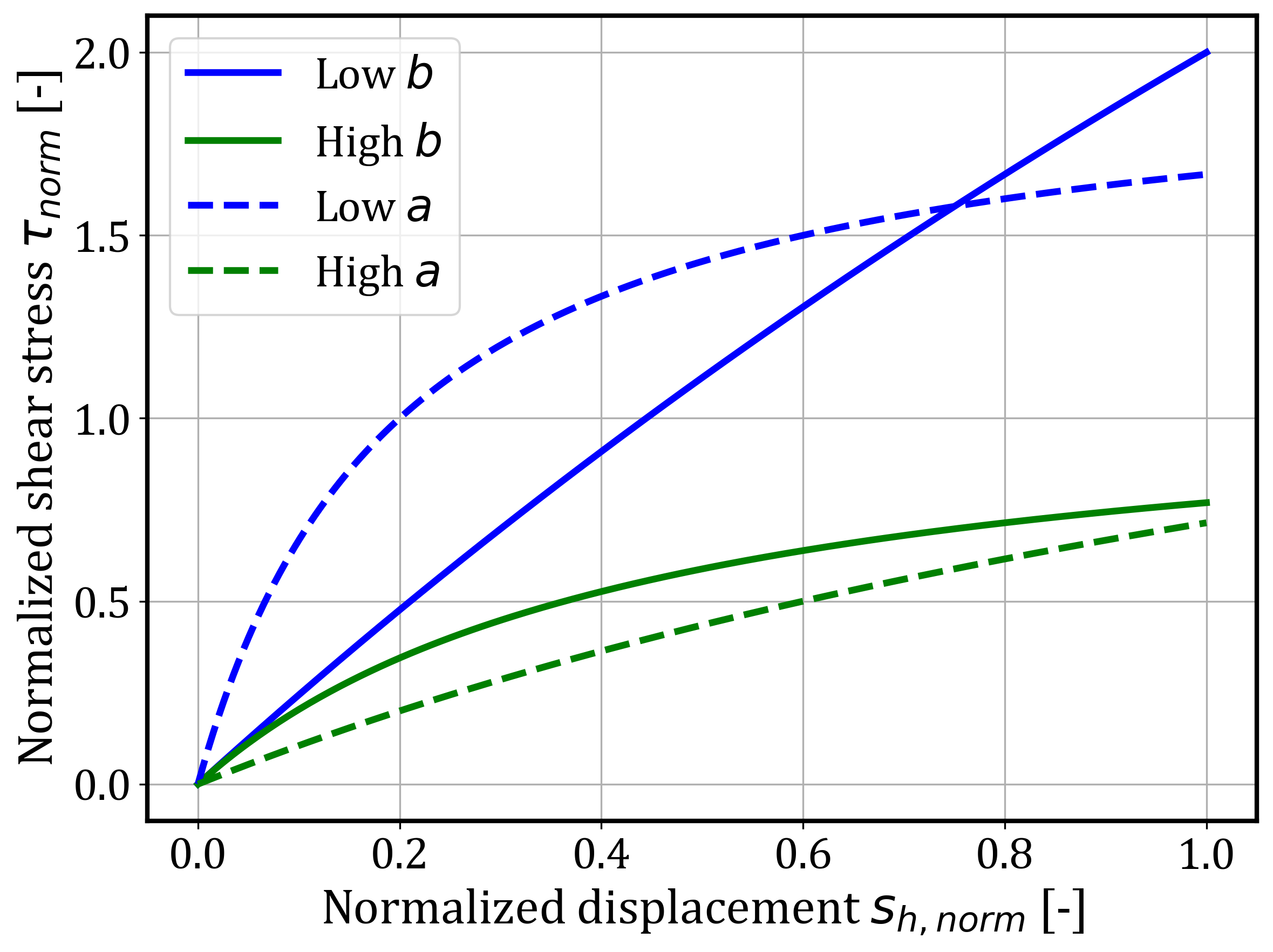
The normalized hyperbolic model developed in this study is governed by two parameters, a and b, which together define the shape of the shear stress–displacement curve. The parameter a influences the initial slope, while b controls how quickly the curve approaches its asymptotic limit.

Figure 6 illustrates the influence of parameters 𝑎 and 𝑏 on the curve shape. Two pairs of curves are shown: one set (solid lines) with different values of 𝑏 and constant 𝑎, and another set (dashed lines) with varying 𝑎 and constant 𝑏. A higher value of 𝑏 causes the curve to approach the peak shear stress more gradually, resulting in a flatter shape. In contrast, a lower 𝑏 leads to faster mobilization and a steeper curve. The initial slope, however, is governed primarily by 𝑎, as will be discussed in Section 4.3. As shown by the dashed lines in Figure 6, a lower value of 𝑎 results in a steeper initial slope, indicating higher initial stiffness. Conversely, a higher value of 𝑎 leads to a more gradual increase in shear stress at the beginning of the curve. These differences illustrate the flexibility of the hyperbolic formulation in capturing various mobilization behaviors observed in direct shear tests. The observed dependency of curve shape on these parameters will be further explored using a normalized stiffness parameter in the following section.

4. 3. Influence of Normalized Secant elastic modulus

To explore how the parameters a and b relate to the mechanical behavior of the material, a normalized secant elastic modulus E_50,norm is introduced. This modulus is defined as the slope between the origin and 50% of the normalized peak shear strength, and is calculated using the Eq. 8:

(8)

Where E_50,norm is the normalized secant elastic modulus, τ_p,norm is the normalized peak shear stress, and s_h,norm is the normalized shear displacement.

Figures 7 and 8 present the empirical relationships between E_50,norm and the parameters a and b, respectively. Both curves were fitted using the following generalized expression:

(9)

Where E_50,norm is the normalized secant elastic modulus and k₁, k₂, k₃, and k₄ are regression constants.

The same form was used to fit the function b(E_50,norm) with a different set of coefficients. Table 1 summarizes the fitted constants k₁ to k₄ for both functions.

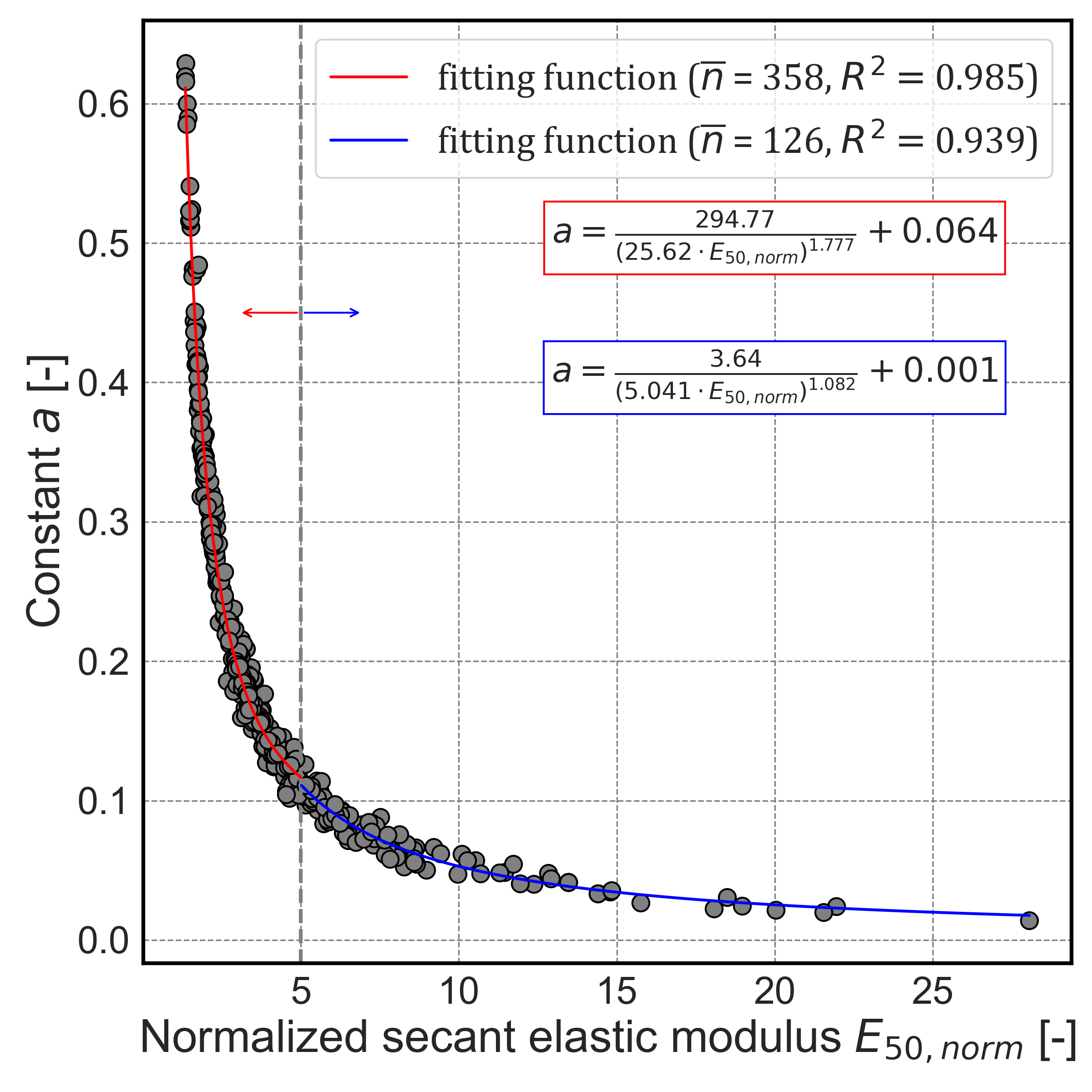
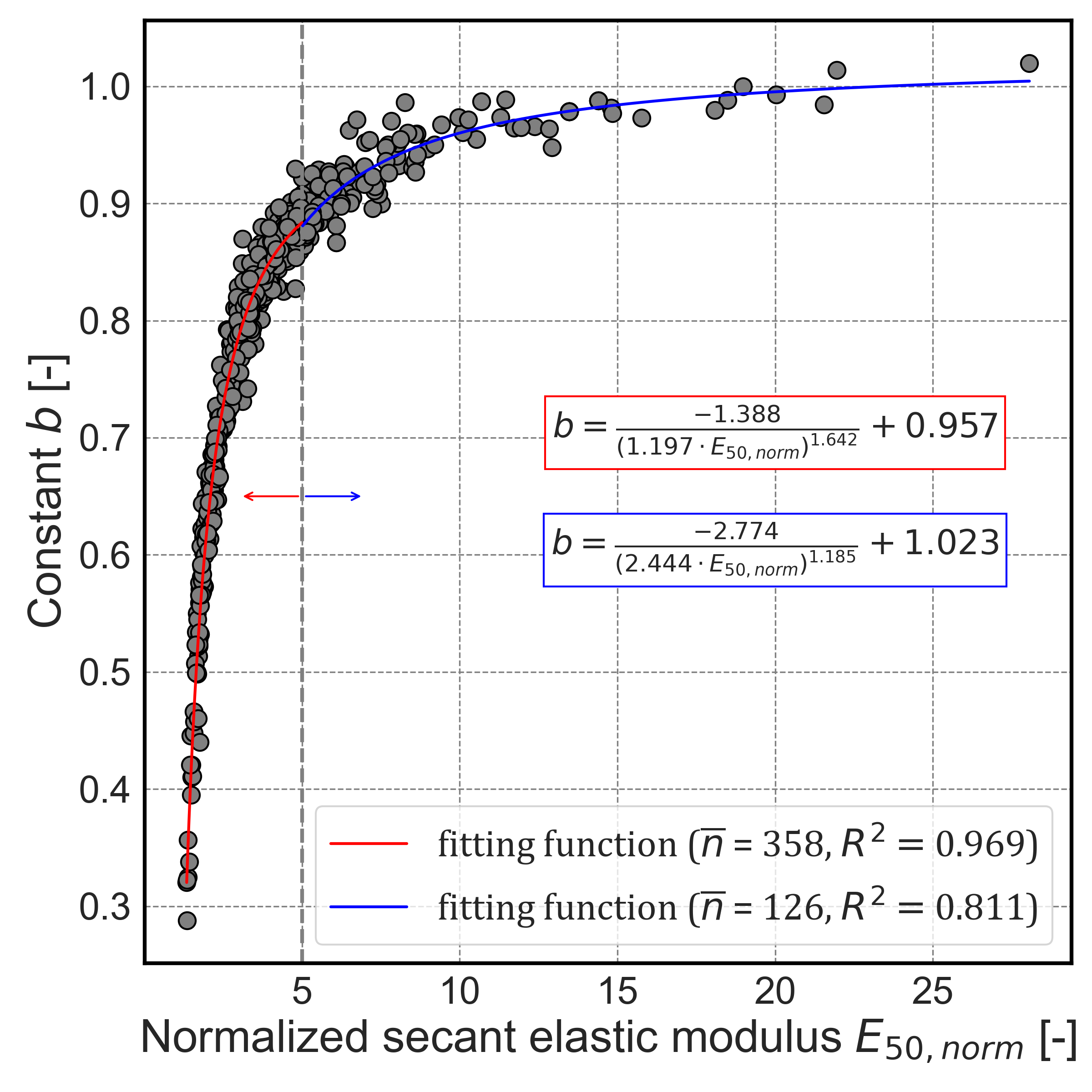
These relationships capture the non-linear dependence between the normalized secant modulus and the curve shape parameters a and b, and demonstrate consistent behavior across a wide range of are valid across a wide range of normalized secant modulus values.

Table 1. Fitted coefficients for the prediction of parameters a and b as functions of E_50,norm, evaluated in two stiffness regions defined by a threshold in E_50,norm.

Param.	Reg.	k1 [-]	k2 [-]	k3 [-]	k4 [-]
a	≤5	294.77	25.62	1.777	0.064
a	>5	3.64	5.041	1.082	0.001
b	≤5	-1.388	1.197	1.642	0.957
b	>5	-2.774	2.444	1.185	1.023

Additionally, the failure ratio R_f was fitted as a function of the normalized secant elastic modulus E_50,norm using a logarithmic expression:

(10)

Where R_f is the failure ratio, α and β are regression coefficients, and E_50,norm is the normalized secant elastic modulus at 50% of the peak shear stress.

This relationship captures the progressive increase in mobilized strength with increasing stiffness. As illustrated in Figure 9, the data exhibit a clear trend. However, a single function was not sufficient to represent the entire dataset accurately.

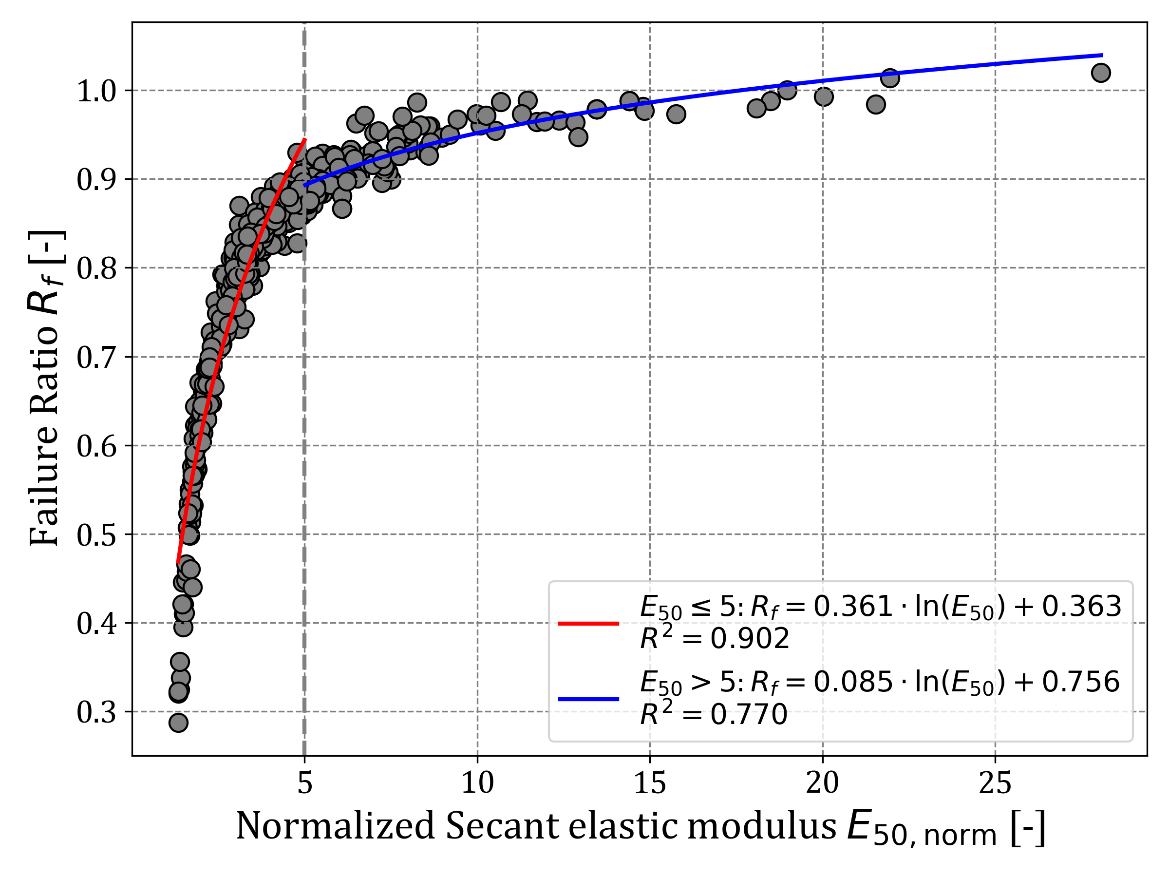
Therefore, a piecewise fitting approach was applied using a threshold at E_50,norm=5, resulting in two separate regressions. The coefficients of determination for the low and high stiffness ranges were R²=0.902 and R²=0.77 respectively.

These results confirm that stiffness plays a key role in controlling not only the curve shape but also the mobilized strength. This finding further supports the development of simplified formulations, such as a direct link between parameters 𝑎 and 𝑏, explored in the next section. These empirical correlations not only provide a mathematical link between curve parameters and stiffness but also reflect fundamental aspects of soil behavior. Specifically, the parameter a is associated with the initial stiffness of the material, while b governs the mobilization rate of shear strength. The normalized secant modulus serves as a practical indicator that integrates both effects, allowing practitioners to anticipate the shape of the shear curve based on early-stage stiffness. This has direct implications for test interpretation, particularly when shear curves are incomplete or truncated in multistage procedures.

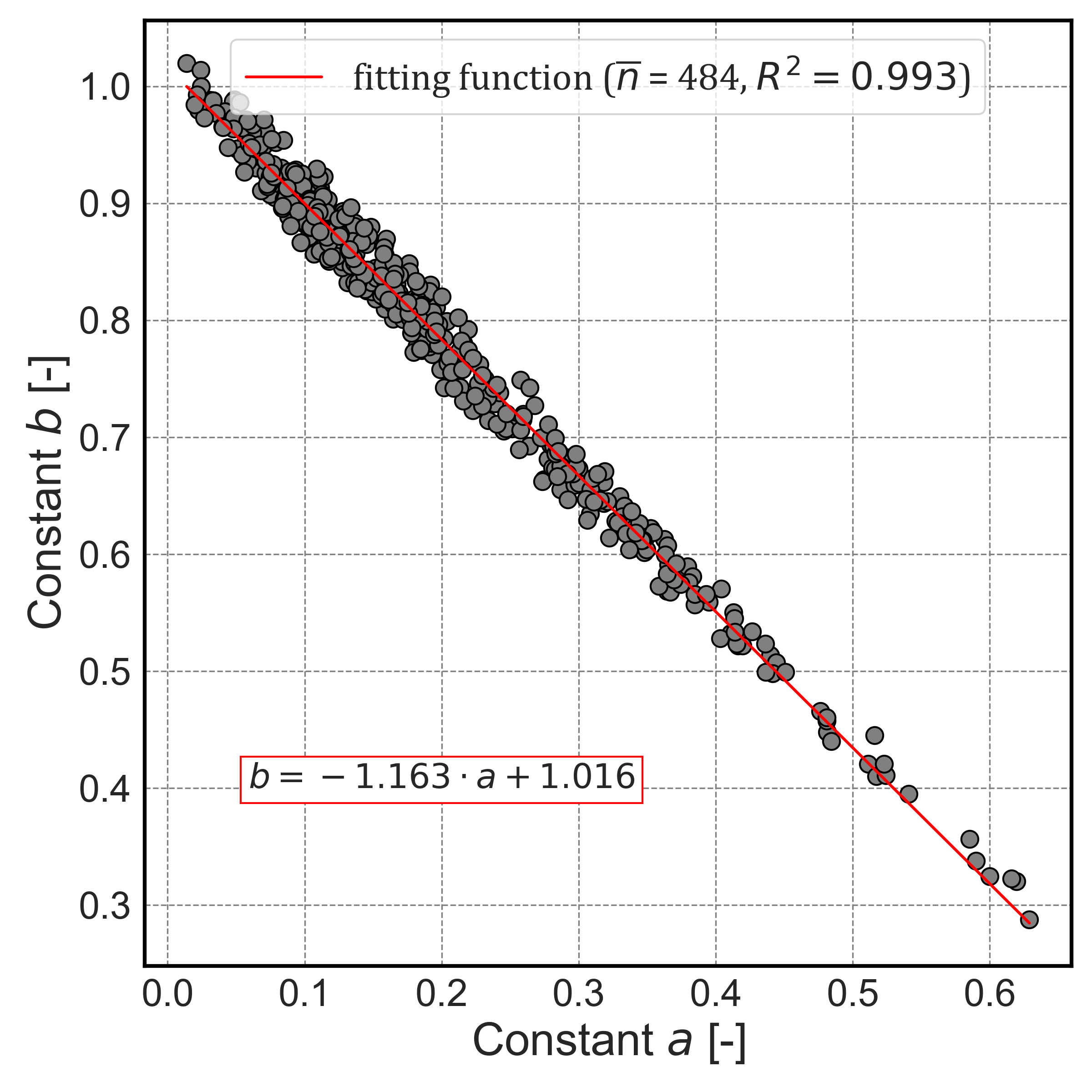
To further simplify the prediction of peak values, a linear relationship between the parameters a and b was observed and fitted as:

(11)

Where a and b are the model parameters from the normalized hyperbolic function, and k₁ and k₂ are regression constants derived from the empirical relationship between the two parameters.

This empirical fit yielded a coefficient of determination of 0.993, indicating a strong correlation. Additionally, based on the normalized condition where τ_p,norm=1 and s_h,norm, the hyperbolic function simplifies to:

(12)

Where a and b are the model parameters describing the shape of the normalized hyperbolic function. This identity reflects the constraint at the peak state, where both the normalized shear stress and displacement are equal to 1.

Figure 10 shows the correlation between a and b, which aligns closely with both the linear regression and the theoretical expression from Eq. 12.

Finally, the potential correlation between b and the normalized initial elastic modulus E_i,norm was evaluated, but no significant trend was identified, as shown in Figure 11. This is likely due to the high sensitivity of E_i,norm to initial measurement noise and device resolution.

4. 4. Soil-Specific Observations

To assess whether the fitted parameters a, b, and the derived failure ratio R_f display consistent trends across different soil types, the results were grouped according to the Unified Soil Classification System (USCS). While the proposed mobilization model is intended to be independent of soil classification, identifying soil-specific tendencies can provide valuable insights for practical application.

The fitted values of R_f, 𝑎, and 𝑏 were analyzed by soil group to identify potential classification-dependent trends. Figures 12 to 15 present boxplots for each of these parameters grouped by USCS classification. In all boxplots, the grey boxes represent the interquartile range (25th to 75th percentile), the red line indicates the median, whiskers extend to 1.5 times the interquartile range, and outliers are plotted as individual points.

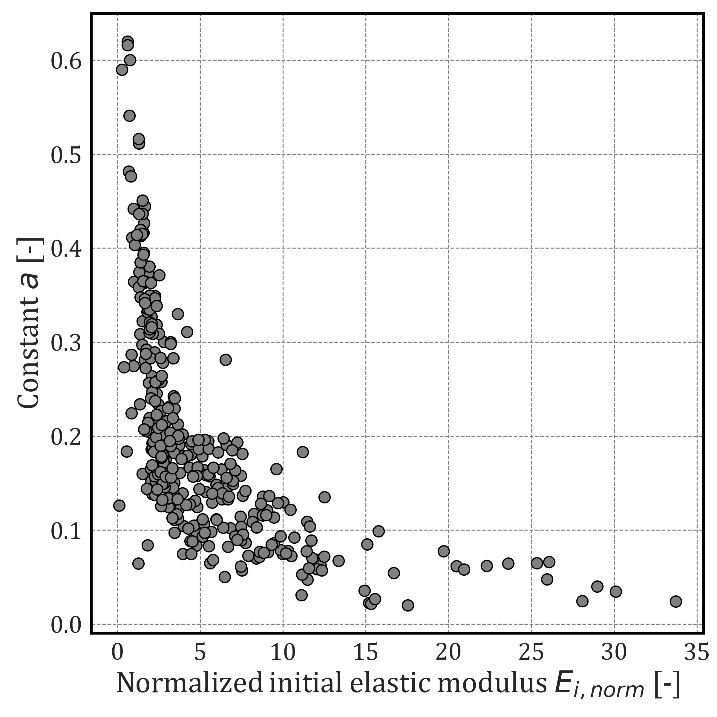
Figure 12 presents boxplots of the failure ratio R_f by soil group. Granular soils such as GP and GW exhibit lower R_f values, with mean values between 0.6 and 0.7.

In these soils, the fitted parameters reveal relatively low 𝑏 and high a values compared to the other soil groups. This combination indicates higher initial stiffness and faster mobilization of shear strength, as illustrated in Figures 13 and 14.

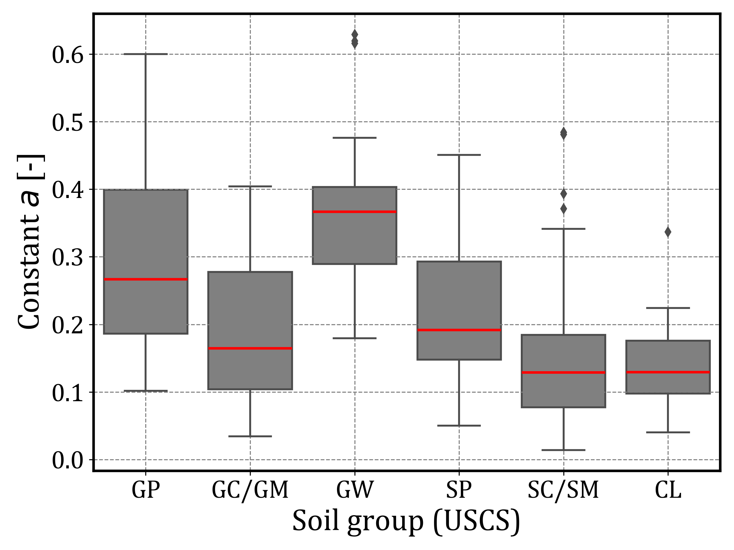
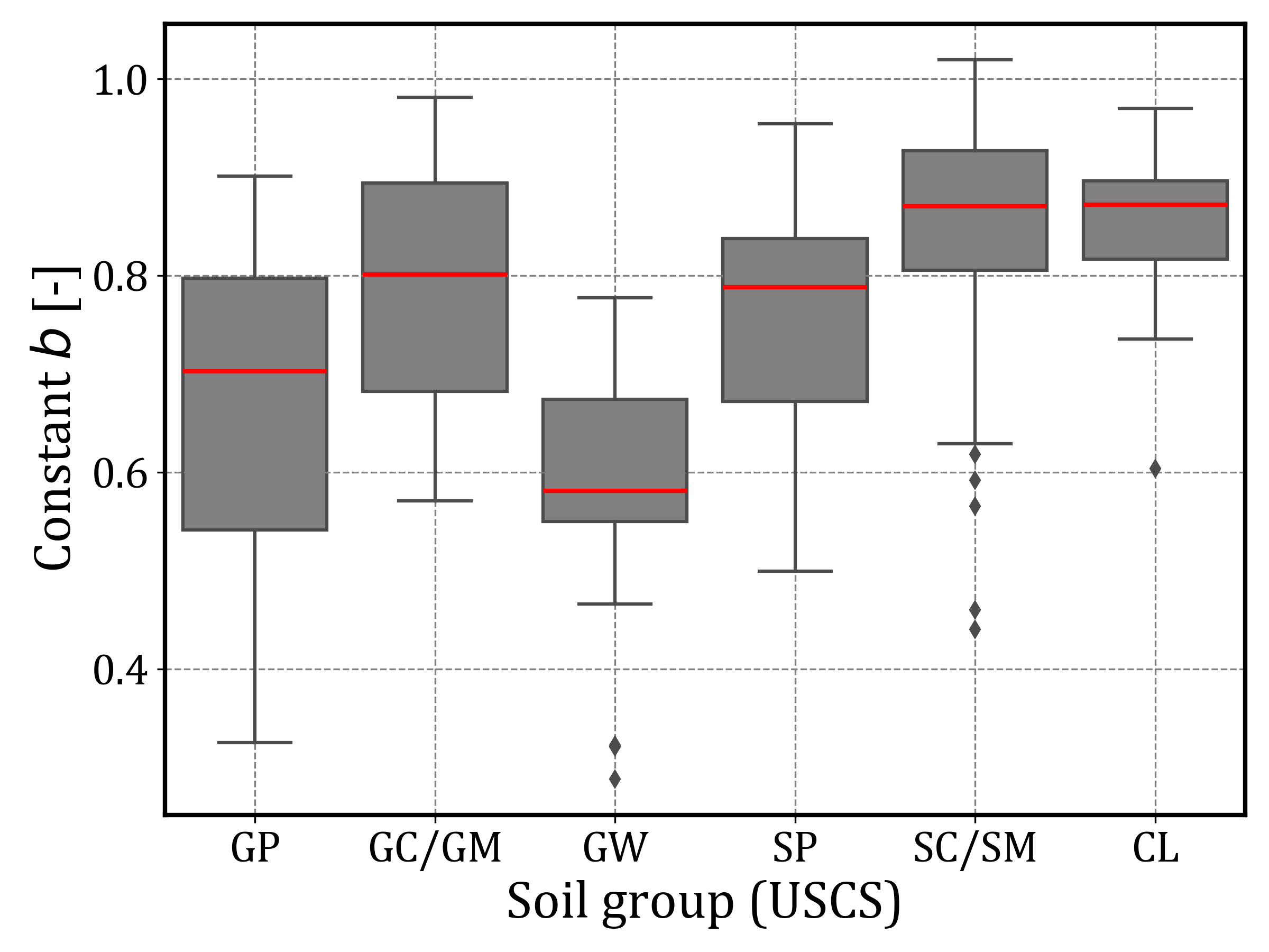
In contrast, fine-grained soils such as CL and SC/SM tend to display higher R_f values, often near 0.9, along with relatively lower a and higher b. This results in more curved-stress-displacement responses and a more gradual mobilization of shear stress at lower stiffness levels. These trends support the interpretation that soils with a significant fines content tend to develop strength more progressively, reflecting the tendency of normally consolidated fine-grained soils to deform gradually and mobilize strength over a longer displacement range.

5. Methodology for predicting peak shear strength

The primary objective of this study is to develop a reliable method for predicting peak shear strength using an algorithm based on the hyperbolic function introduced earlier, with the parameters a and b derived in section 4.3.

5. 1. Overview of the Prediction Algorithm

This algorithm processes shear stress and shear displacement data up to a specific level of mobilization, normalizes the data, fits them to the hyperbolic function and then extrapolates the data to estimate the peak values.

However, in multistage testing, the first and second shearing phases are terminated before reaching the peak, leaving the maximum shear stress (τ_p) and the corresponding shear displacement at peak (s_h,p) unknown.

Since normalization requires these peak values, a search algorithm is needed to estimate τ_p and s_h,p, based on the available curve segment.

5. 2. Derivation of Key Parameters

The critical parameters required for the algorithm are:

• a_F, b_F: Constants determined through regression based on known data, using Eq. 7.
• a_E: Constant derived from E_50,norm (determined from known data) using the empirical Eq. 9, with k₁=294,77, k₂=25,62, k₃=1,777, and k₄=0,064 for E_50,norm≤5 and with k₁=3,64, k₂=5,041, k₃=1,082 and k₄=0,001 for E_50,norm>5
• b_E: Constant determined from the relationship between the constants a and b, using the empirical Eq. 11, with k₁=-1,163 and k₂=1,016.

5. 3. Optimization Procedure and Error Minimization

This algorithm estimates the unknown values of τ_p and s_(h,p) from the available portion of the normalized shear stress-displacement curve by identifying the best-fit parameters a_Fand b_F. These fitted values are then compared with the expected parameters a_E and b_E, which are derived from the normalized secant elastic modulus E_50,norm using Eqs. 9 and 11.

To evaluate the accuracy of each prediction, the algorithm computes the mean squared error (MSE) between the fitted and estimated parameters, as defined in Eq. 13:

(13)

Where MSE_mean is the mean squared error, a_F and b_F are the constants determined through regression using Eq. 7, and a_E and b_E are derived from the empirical Eqs. 9 and 11.

A stochastic optimization method based on differential evolution is applied to explore various combinations of τ_P and s_h,p, aiming to minimize the MSE. This search process iteratively adjusts the assumed peak values until the best agreement is found between the empirical model and the measured data segment.

The boundaries for τ_P and s_h,p are predefined based on practical considerations and prior knowledge from fully mobilized curves, particularly those obtained in the third shearing phase in multistage tests. This constraint ensures that the optimization remains physically meaningful and computationally efficient.

5. 4. Validation and Model Fitting

To evaluate the accuracy of the proposed model in predicting the peak shear strength τ_P a relative error analysis was performed on the full dataset of 484 direct shear tests. The relative error (RE) was calculated according to Eq. 14, comparing the predicted and measured values of τ_P.

(14)

Where RE is the relative error in percentage, τ_p,pred is the predicted peak shear stress, and τ_p is the measured peak shear stress.

Figure 15 illustrates the distribution of relative errors for different termination thresholds of the shear curve. Each density function represents a normal distribution fitted to the prediction error at a specific percentage of the peak displacement s_h,p. The curves demonstrate that the prediction error tends to decrease as the available portion of the mobilization curve increases, and that reliable predictions can be achieved even when the test is stopped early.

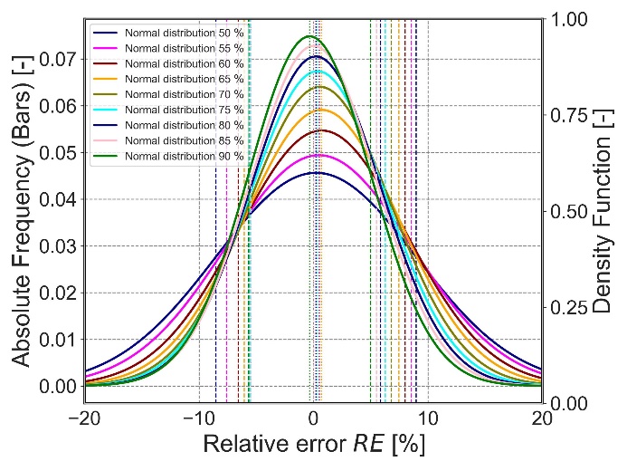
Figure 16 summarizes the percentage of tests for which the prediction error exceeds specific relative error (RE) thresholds (i.e., 5 %, 8 %, 10 %, and 15 %), plotted against the termination point expressed as a percentage of the shear displacement at peak.

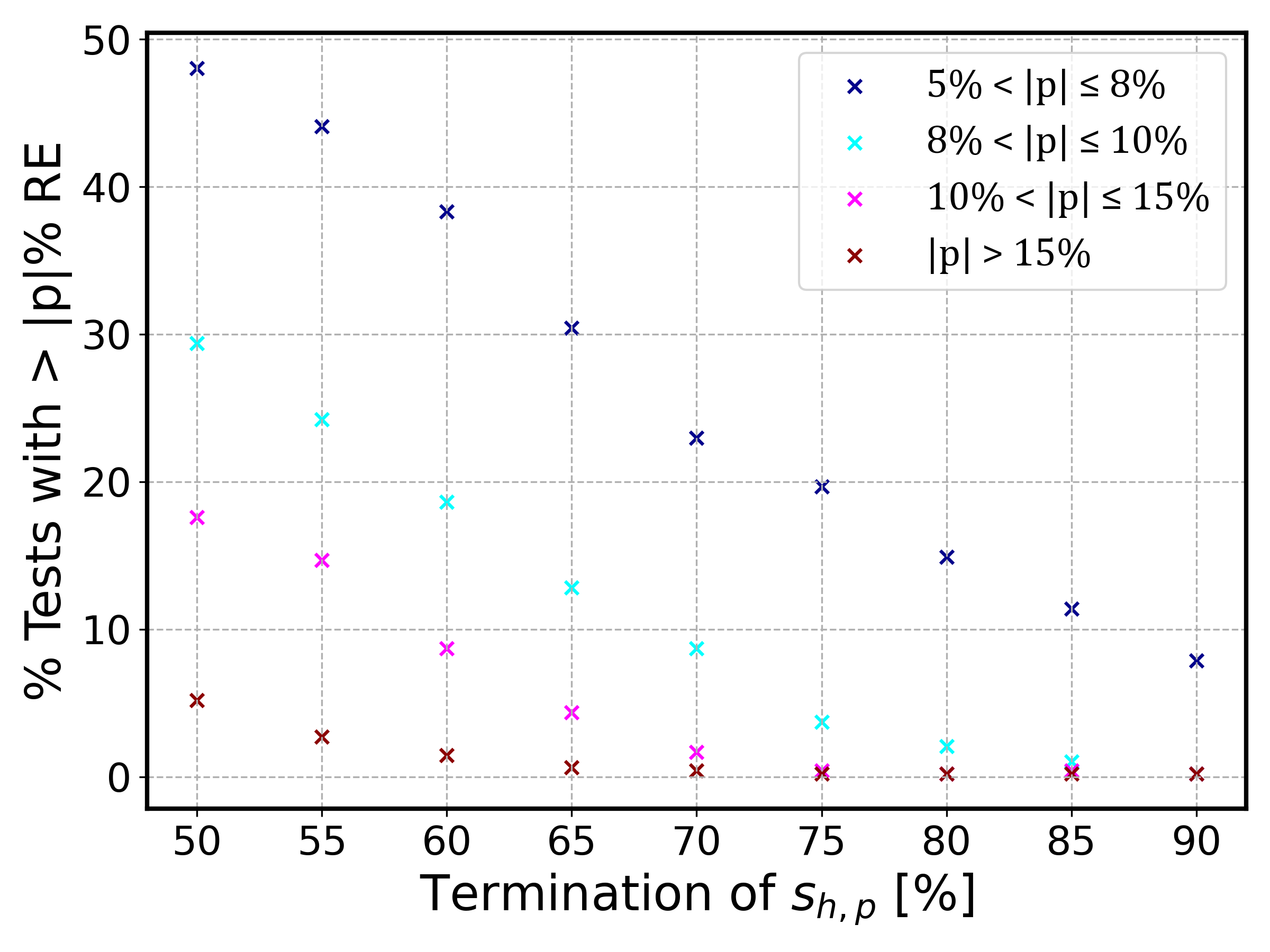
The proportion of tests with large prediction errors consistently decreases as the level of mobilization increases, reinforcing the applicability of the method to truncated shear tests. Notably, even when only 60 % of the peak displacement is mobilized, the majority of predictions fall within an error range below 10 %.

These results confirm the robustness of the normalized hyperbolic model in estimating τ_p from incomplete data, and support its use in multistage test configurations where full mobilization is intentionally avoided.

6. Practical Application of the Model

In multistage direct shear testing, it is common for the initial stages to be interrupted before the peak shear strength is fully mobilized. This occurs intentionally to preserve specimen integrity for subsequent loading stages. As a result, the shear stress–displacement curves in the early phases lack a clear peak, making it difficult to determine shear strength parameters directly.

The proposed model provides a practical solution by fitting the available portion of the curve and extrapolating the expected peak shear strength. This approach is particularly useful in multistage procedures where each shearing phase is intentionally halted before full mobilization, followed by a complete reset of the horizontal displacement. This includes procedures such as MSB, previously described in detail by Toledo Arcic (2025), where early termination is applied to preserve specimen structure while ensuring continuity between stages.

6. 1. Experimental Setup and Test Conditions

All tests were performed using a large-scale shear box with internal dimensions of 30 × 30 cm and a height of 20 cm. The soil specimens were compacted in three layers to achieve uniform density and homogeneity, following the standard Proctor density ρ_pr and optimum water content w_pr.

The analysis shown in Figures 17-19 corresponds to MIX 3, classified as ST* (strongly clayey sand) according to DIN 18196 [17]. This mixture has a fines content of 24.1%, 52.2 % sand, and 23.7% gravel, with a specific gravity G_s=2.647, a Proctor maximum dry density ρ_pr=2.180 g/cm³, and an optimum water content w_pr=7.96%.

All specimens were prepared and tested by the same operator to minimize human error and ensure consistency. The normal stresses applied were 100, 200, and 400 kPa, consistent across both singlestage and multistage configurations to ensure comparability of the resulting shear curves.

6. 2. Results and Model Comparison

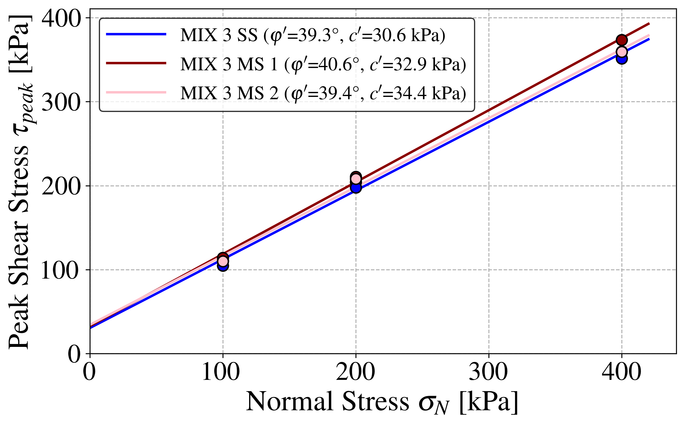
Figure 17 illustrates this application using two multistage tests (shown in red and pink), in which the first and second stages were terminated before peak strength was reached. For comparison, singlestage test curves conducted under the same normal stress conditions are shown in blue.

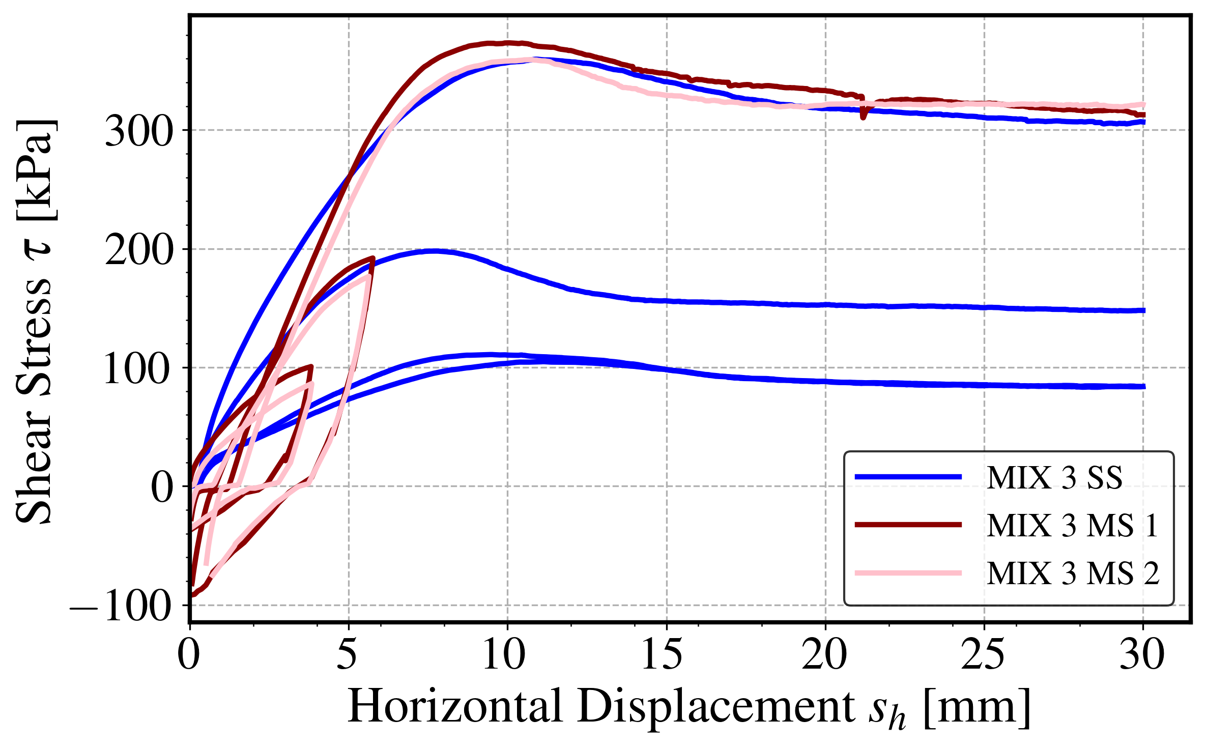
Figure 18 presents the corresponding failure envelopes derived without correcting for peak shear strength. As seen, the omission of the correction leads to an overestimation of the friction angle and an underestimation of cohesion.

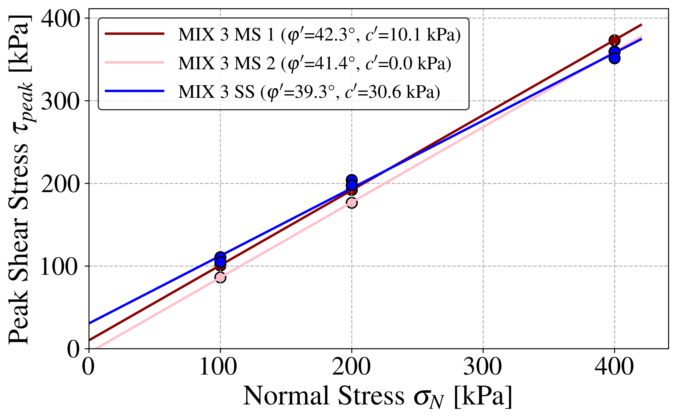
To address this, the extrapolation model developed in this study was applied to estimate the expected peak shear strength in the incomplete first and second shearing phases. The corrected failure envelopes, shown in Figure 19, demonstrate that the results from the multistage tests closely align with those obtained from singlestage tests. This confirms the model’s capability to harmonize strength estimation across different testing procedures.

6. 3. Implications for Practice

This practical application significantly enhances the efficiency and reliability of multistage shear testing, especially for mixed or fine soils where full mobilization in each phase may not be feasible. The model enables more robust data interpretation under realistic laboratory constraints.

7. Conclusion

This study introduces a new model for predicting the shear stress and shear displacement at the peak state in direct shear tests. The model uses the initial data from the stress-displacement curve and incorporates empirical methods to predict them. It normalized the shear stress-displacement curve up to the peak and fitted the data to a Kondner function. Developed initially for drained triaxial tests, this approach forms the foundation for several material models, including the Hardening Soil or Duncan-Chang models.

The two constants, a and b are fundamental to the model, with a strongly correlating with the normalized secant modulus at 50% of the peak shear stress, while b demonstrates a linear relationship with a. By applying these two constants and a newly developed stochastic algorithm based on differential evolution, the model accurately predicts the peak shear strength and the shear displacement at peak.

The model was validated using 484 direct shear tests on different materials to determine the constants a and b, and the results were evaluated against known peak states. After analyzing data from different soil types, the parameters proved applicable across different soil groups. The goal is to establish the optimal stopping point during the shear test as a basis for multistage tests. To achieve this, mobilization curves with displacements between 50% and 90% of the peak shear displacement were compared with the predictions from the new model. The evaluation relied on the stochastic analysis of normal distributions and their deviations, ensuring prediction accuracy within defined limits.

Overall, the model provides a practical and reliable tool for improving the interpretation of direct shear test data. It enhances the efficiency of multistage procedures by allowing early termination without compromising the accuracy of shear strength parameters.

Future research will focus on developing methods to determine the shear strength of soils using multistage tests, aiming to achieve results equivalent to those from singlestage tests. Defining the optimal stopping criterion during the shearing phase is crucial for this goal. The results presented here are based on tests conducted with compacted samples. Additional adjustments will be needed to account for other influencing factors, such as aging or structure.

Acknowledgements

The Federal Ministry for Economy Affairs and Climate Action BMBF (Project number 49VF230003) and Bank of Saxony SAB (Project number 100604731) supported this research financially.

References

[1] S. Nam, M. Gutierrez, P. Diplas and J. Petrie, "Determination of the shear strength of unsaturated soils using the multistage direct shear test," in Engineering Geology, 2011, vol. 122, pp. 272-280.
View Article
[2] D. Hormdee, N. Kaikeerati and P. Angsuwotai, "Evaluation on the results of multistage shear test," in International Journal of GEOMATE, 2012, vol. 2, pp. 140-143.
[3] H. S. Saeedy and M. A. Mollah, "Application of Multi-Stage Triaxial Test to Kuwaiti Soils," in: Donaghe, R.T., Chaney, R.C. and Silver, M.L., Eds., Advanced Triaxial Testing of Soil and Rock, ASTM, Philadelphia. 1988, pp. 363-375.
[4] D. Kotsanis, P. P. Nomikos, D. Rozos and A. I. Sofianos, "Multistage triaxial testing of various rock types: A case study of East Attica Prefecture, Greece," in Procedia Structural Integrity, 2018, vol. 10. pp. 112-119.
[5] A. Vakilinezhad1 and N. K. Toker, "Application and comparison of multistage triaxial compression test procedures on reconstituted Ankara clay," in Proceedings of the 3S Web of Conferences 544 IS-Porto 2023, 2024, vol. 544.
[6] M. J. Toledo Arcic, "Entwicklung einer datenbasierten Steuerung für Scherversuche in Mehrstufentechnik," in Tagungsband der 38. Baugrundtagung, Forum für junge Geotechnik-Ingenieure und -Ingenieurinnen, Dresden, Germany, 2024, pp. 39-46.
[7] R. L. Kondner, "Hyperbolic stress-strain response: cohesive soils," in: J. Soil Mech. Found., ASCE 89 (SM1), 1963, pp. 115-143.
[8] J. M. Duncan and C. Y. Chang, "Nonlinear analysis of stress and strain in soil," in: Journal of the Soil Mechanics and Foundations Division. ASCE. 1970, Vol. 96. Nr. 5. pp. 1629-1653.
[9] R. Obrzud and A. Truty, “The Hardening Soil Model– A Practical Guidebook,” Zace Services Ltd, Software Engineering, Switzerland, 2018. [Online]. Available:
[10] T. Schanz, P. A. Vermeer and B. G. Bonnier, "The Hardening Soil Model: formulation and verification," in: Beyond 2000 in Computational Geotechnics - 10 years of PLAXIS, Balkema, 2000.
[11] T. M. Tharp and M. G. Scarbrough, "Application of hyperbolic stress-strain models for sandstone and shale to fold wavelength in Mexican Ridges Foldbelt," in J. Struct. Geol. 1994, 16(12), pp. 1603-1618.
[12] J. M. Duncan, "Hyperbolic stress-strain relationships," in: Limit Equilibrium, Plasticity and Generalized Stress-Strain in Geotechnical Engineering (edited by Yong, R. K. & Ko, H.-Y.). Am. Soc. Civ. Engr., New York. 1981, pp. 443--460.
[13] J. Habimana, V. Labiouse and F. Decoeudres, "Geomechanical characterisation of cataclastic rocks: Experience from the Cleuson-Dixence project," in: Int. J. Rock Mech. Min. Sci. 2012, 39(6), pp. 677-693.
[14] Y. P. Vaid, "Effect of consolidation history and stress path on hyperbolic stress-strain relations," in: Canadian Geotechnical Journal, 1985, 22. pp. 172-176.
[15] M. J. Toledo Arcic, A. Mehrpajouh, C. Lauer, M. Pamler und J. Engel, "Komplexe Bewertung bodenmechanischer Versuche zur Ermittlung von Kennwerten," Konstruktiver Ingenieurbau, Bd. 06, pp. 5-10, 2022.
[16] M. J. Toledo Arcic, "Comparison of different methods for conducting multistage direct shear tests," in: Proceedings of the 10th World Congress on Civil, Structural, and Environmental Engineering (CSEE 2025), Barcelona, Spain - April, 2025.
[17] DIN 18196:2023-02. "Earthworks and foundations - Soil classification for civil engineering purposes," Deutsches Institut für Normung, Berlin, Germany.
[1] S. Nam, M. Gutierrez, P. Diplas and J. Petrie, "Determination of the shear strength of unsaturated soils using the multistage direct shear test," in Engineering Geology, 2011, vol. 122, pp. 272-280. View Article
[2] D. Hormdee, N. Kaikeerati and P. Angsuwotai, "Evaluation on the results of multistage shear test," in International Journal of GEOMATE, 2012, vol. 2, pp. 140-143. View Article
[3] H. S. Saeedy and M. A. Mollah, "Application of Multi-Stage Triaxial Test to Kuwaiti Soils," in: Donaghe, R.T., Chaney, R.C. and Silver, M.L., Eds., Advanced Triaxial Testing of Soil and Rock, ASTM, Philadelphia. 1988, pp. 363-375. View Article
[4] D. Kotsanis, P. P. Nomikos, D. Rozos and A. I. Sofianos, "Multistage triaxial testing of various rock types: A case study of East Attica Prefecture, Greece," in Procedia Structural Integrity, 2018, vol. 10. pp. 112-119. View Article
[5] A. Vakilinezhad1 and N. K. Toker, "Application and comparison of multistage triaxial compression test procedures on reconstituted Ankara clay," in Proceedings of the 3S Web of Conferences 544 IS-Porto 2023, 2024, vol. 544. View Article
[7] R. L. Kondner, "Hyperbolic stress-strain response: cohesive soils," in: J. Soil Mech. Found., ASCE 89 (SM1), 1963, pp. 115-143. View Article
[8] J. M. Duncan and C. Y. Chang, "Nonlinear analysis of stress and strain in soil," in: Journal of the Soil Mechanics and Foundations Division. ASCE. 1970, Vol. 96. Nr. 5. pp. 1629-1653. View Article
[9] R. Obrzud and A. Truty, “The Hardening Soil Model– A Practical Guidebook,” Zace Services Ltd, Software Engineering, Switzerland, 2018. [Online]. Available: View Article
[11] T. M. Tharp and M. G. Scarbrough, "Application of hyperbolic stress-strain models for sandstone and shale to fold wavelength in Mexican Ridges Foldbelt," in J. Struct. Geol. 1994, 16(12), pp. 1603-1618. View Article
[13] J. Habimana, V. Labiouse and F. Decoeudres, "Geomechanical characterisation of cataclastic rocks: Experience from the Cleuson-Dixence project," in: Int. J. Rock Mech. Min. Sci. 2012, 39(6), pp. 677-693. View Article
[14] Y. P. Vaid, "Effect of consolidation history and stress path on hyperbolic stress-strain relations," in: Canadian Geotechnical Journal, 1985, 22. pp. 172-176. View Article
[16] M. J. Toledo Arcic, "Comparison of different methods for conducting multistage direct shear tests," in: Proceedings of the 10th World Congress on Civil, Structural, and Environmental Engineering (CSEE 2025), Barcelona, Spain - April, 2025. View Article