International Journal of Civil Infrastructure (IJCI)

ISSN: 2563-8084

1. Introduction

In many ground investigation projects, thin layers of soft soils embedded with relatively denser materials (or vice versa) are encountered. At or around the borders between the layer with different consistencies never can a sharp change in the cone penetration test (CPT) readings be observed, particularly in the cone tip resistance (q_c). Influence of these thin layers can affect the results even when the CPT cone has still a remarkable distance to them. The affected zone (also named transition zone, TZ) can reach to 10-20 times cone diameter (‎[1]). ‎[2] experimentally showed that q_c is influenced by the layers not only ahead of the CPT cone but also behind it.

‎[3] (NCEER) proposed a method for correction of CPT results in a denser soil interbedded between two softer layers in which the correction factor was a function of the dense layer thickness. ‎[4] suggested that the transition zone corrections should not be uniformly applied over depth. Later ‎[5] modified the method suggested in the NCEER by mathematically relating the correction factor to the shortest distance to the soft-to-dense boundary. That means the further from the dense-to-soft boundaries the q_c is measured, the less impact has occurred, hence less correction would be needed. With numerical axisymmetric penetration studies on various combinations of two-layered soils, ‎[6] showed that when entering from soft to dense soil, the border can be detected by CPT from a larger distance compared to when entering from dense to soft soil. They also stated that the cone senses the border farther ahead than behind. ‎[7] introduced a so called Inverse Filtering, an iterative procedure, to estimate the unaffected q_c and sleeve friction (f_s) with sharp transitions. Several other researchers also investigated the CPT results in layered soils both experimentally (e.g., chamber test: ‎[8], ‎[9] and ‎[10]; and centrifuge test: ‎[11]) and numerically (e.g., cavity expansion: ‎[12]; and axisymmetric penetration analysis: ‎[13], ‎[14] and ‎[15]).

In this research series of models with one soft layer (with various thickness, h_s) embedded in dense soil were numerically simulated. The CPT cone selected in this work had diameter and tip angle of 35.7 mm and 60°, respectively. The Stiffness Ratio (R_s) (i.e., stiffness of soft soil (E_s) divided by that of the surrounding dense soil (E_d)) was another parameter whose sensitivity was studied over values from 0.042 to 0.833. Finally, the outcomes were discussed based on which a simplified correction method was introduced to estimate the actual (unaffected) q_c values.

2. Numerical Studies

2. 1. Modelling CPT

Several studies have attempted to numerically model CPT (e.g., ‎[16], ‎[17], ‎[18], ‎[19] and many others). The most critical challenges that such modelling face are the complexity of the model due to the large deformations (mesh distortion) and the solution schemes (stress and deformation history in the soil, selecting an appropriate material model, interfaces, tension in soil, etc.).

Considering a continuous penetration of the CPT cone into the soil with a constant velocity (usually 20 mm/s) in the numerical modelling is a more realistic approach. However, regarding the complexity of situation, in this study a simplified method of modelling CPT was used, in which the cone does not penetrate throughout the depth in one run, but only 20 mm at consecutive and independent steps. First, the CPT cone and rod was modelled at a given depth. In the next phase of modelling, to simulate the penetration, a vertical displacement of 20 mm in one second was imposed on top of the rod. The mobilized vertical stress at top of the rod was considered as an indicator for the q_c. Then the CPT rod and cone was extended (re-modelled) to the next measurement level, the mesh was updated, and another 20 mm displacement was imposed. The same procedure was repeated to cover the whole investigation depth. The friction between CPT and soil was ignored and the CPT-to-soil interface could transfer only normal stress between the two bodies. The modelling was carried out using Plaxis 2D v.21.

This modelling approach fails to capture some aspects of the CPT test. In order to minimize the effect of the modelling limitations, the calculated vertical stress in the rod (here named σ_c) should not be considered directly as q_c, but can be normalized by a reference σ_c (σ_c,ref) calculated in the same way. In section ‎3 the normalization procedure is explained.

2. 2. Studied Conditions

In this study CPT test, with the above-mentioned modelling concept, was modelled in layered soils. The CPT cone was 35.7 mm in diameter and 60° in tip angle (one of most widely used cone types), and the ground consisted of a soft layer with various thicknesses embedded in a denser soil. Middle of the soft layer, however, was fixed in all models. The studied thicknesses of the soft layer were h_s = 50, 100, 200 and 300 mm. Depths of CPT penetration were selected so as to cover well above and below the soft later. Axisymmetric models with 250 mm width were developed to simulate the geometries as illustrated in Figure 1.

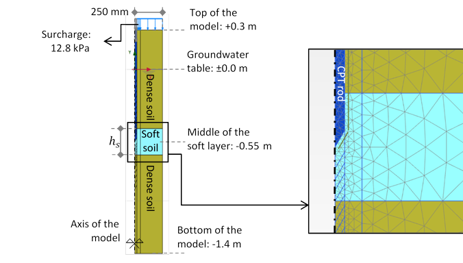
The assigned soil model was Mohr-Coulomb for both soils. Moduli of elasticity of the soft and dense soils (E_s and E_d) as well as the stiffness ratio (R_s=E_s/E_d) are listed in Table 1. The assumed shear strength parameters were φ=32° and c^'=5 kPa for dense soil and φ=25° and c^'=10 kPa for soft soil (usually a silty soil), both with saturated and unsaturated density of 17 and 16 kN/m3. The material assigned to the CPT rod was linear elastic with modulus of elasticity of 200 GPa (modulus of elasticity of steel). A surcharge of 12.8 kPa represented an actual depth of 0.8 m for top of the model.

Table 1. Moduli of elasticity of the studied conditions.

Es[MPa]	Ed[MPa]	Rs[-]
0.5	12	0.042
1	12	0.083
2	12	0.167
3	12	0.250
4	12	0.333
6	12	0.500
8	12	0.667
10	12	0.833

3. Results and Discussions

3. 1. Outcomes of Calculations

In this study the mobilized stress in the rod, denoted by σ_c (or calculated q_c) may not be 100% equal to the field q_c. The difference between σ_c and q_c lies within the modelling limitations. For example the lateral displacement of the soil due to downward penetration of the cone (which increases the stiffness in hardening soils) is missing. Another imperfection is not taking the stress history of the previous penetration steps into consideration. Moreover, the localized fractures occurring in the soil around an advancing CPT cone cannot be fully modelled in the FEM analysis. In order to minimize the modelling limitations, the calculated σ_c values of the layered soil were normalized by σ_c of the homogeneous condition (only dense soil).

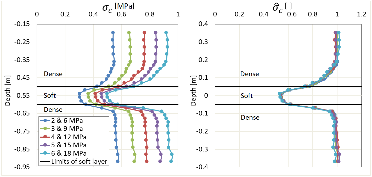
In Figure 2 the concept of normalization is presented. The calculated σ_c (with the assumptions mentioned in section ‎2) are presented in Figure 2(a) for E_s of 2, 3, 4, 5 and 6 MPa and a constant value of 0.333 for R_s (i.e., E_d = 6, 9, 12, 15 and 18 MPa). In Figure 2(b), σ_c values are normalized (hereafter named ) by dividing them by σ_c of dense soil with the corresponding E_d (same calculation procedure but without presence of the soft layer). Please note that in this graph, the zero depth is shifted to the center of the soft layer. As these analyses clearly show, the governing parameter affecting is R_s (the stiffness ratio). Changes in E_d and E_s have no influence on as long as R_s is fixed; that is the reason why in this research a constant value of 12 MPa for E_dwas selected for all models, while R_s was ranging from 0.042 to 0.833.

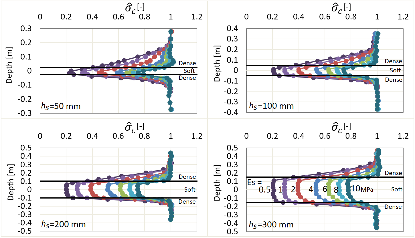
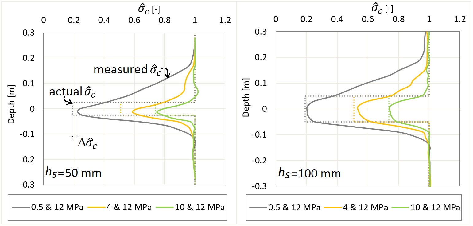
In Figure 3 values are plotted versus depth (zero depth at center of the soft layer) with four different soft layer thicknesses (h_s) and the moduli of elasticities as listed in Table 1. In some points there is minor unevenness in the results which are not expected in an idealized numerical simulation. This effect is due to influence of meshing quality on the results. As it can be seen in Figure 1 the meshes’ shape and size slightly differ from point to point where the tips of CPTs were modelled.

The lower R_s was, the larger drop was observed in the . For h_s of 300 mm (and logically >300 mm) the reaches to an almost constant value in the soft soil. That means the Transition Zones (TZ, where the results were affected) inside the soft layer do not overlap for that thickness. In general, the extension of the TZ in the dense soil was larger than that in the soft soil (also stated by ‎[2] and ‎[6]). Regarding the results in the upper and lower dense soils, as also confirmed by other researchers (e.g., ‎[6]), the TZ was wider in the upper dense soil compared to the lower one. Moreover, the extension of the TZ in the dense soil was a function of h_s and -as mentioned- R_s.

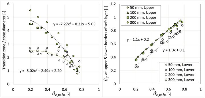
Extension of the TZ can be visually identified and measured for different conditions. In Figure 4(a) the TZ divided by the cone diameter (d_c=35.7 mm) is plotted against minimum (_,min)). The TZ in the upper and lower dense soils are shown by green and white markers, respectively. Unlike R_s, _,min is a parameter measurable from the results which can be correlated to R_s (see Figure 2).

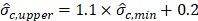
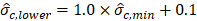
The upper and lower TZ seems to be a function of the _,min. The equations proposed based on the best fit are given on the graph (Eqs. 1 and 2). These formulas allow us to estimate the extend of TZ using the measured _,min. Dependency of TZ on h_s is less pronounced and can be ignored for the sake of simplicity.

In Figure 4(b) values calculated at upper and lower limits of the soft soil (the black horizontal lines in Figure 3) are drawn _,min. Clearly there is no meaningful relation between the at the borders of soil layers and h_s, whereas a linear dependency to the _,min can be observed with the equations suggested on the graph (Eqs. 3 and 4).

(1)

(2)

(3)

(4)

value inside the soft layer was also found to be a function of h_s and R_s. For the sake of place, in Figure 5 is presented only for two h_s and three R_s values. The solid curves show the measured (calculated in the layered soil) and the dotted lines are the actual (calculated in homogeneous soil either only soft or only dense, hence no thin-layer effect). As it can be seen, the thinner the soft layers is, the larger the difference between the measured and the actual in the soft layer will be. Dependency of this difference on h_s, however, is not consistent. The maximum difference took place where the was around 0.55, whereas, for larger and smaller values, the measured and actual in the soft layer were closer.

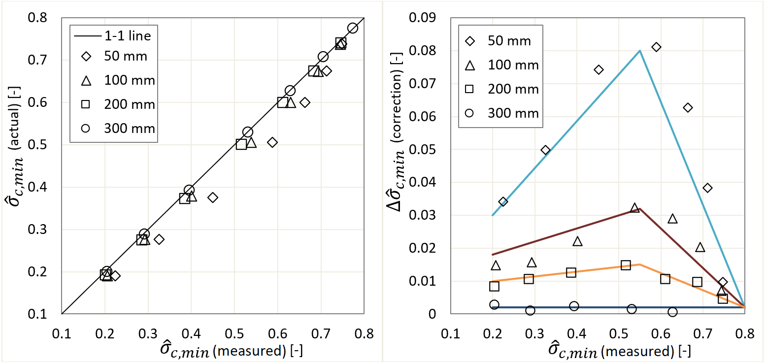
In Figure 6(a) the actual and measured are compared. As mentioned, for large and small , the measured and actual are almost on the 1-1 line, while in between the deviation is at its maximum. In Figure 6(b) the markers show the difference between the measured and actual in the soft layer (∆), and the straight lines simplify their trends.

3. 2. Proposed Correction Procedure

In this paper a thin-layer correction method is proposed trying to back-calculate the actual q_c (unaffected by presence of an embedded soft layer) from the results measured on site. As mentioned earlier, in this study the calculated vertical stress in the CPT rod (σ_c) was considered as an indicator of q_c. σ_c was later normalized by σ_c of dense soil only, as a reference value. Likewise in a real CPT test done on such a ground (a soft layer embedded within denser soil), we can normalize q_c. Similar to the normalization concept of σ_c, the reference value for normalizing q_c could be the q_c before or after the cone senses the soft layer. Changes in the calculated and measured mobilized resistances in a CPT rod are expected to follow a similar trend. Therefore, (normalized q_c) and the are supposed to be in a same range and trend as both are normalized by their own quantities in the dense soil.

For real test results containing several soft and dense layers, the whole correction process should be repeated for every steep decrease or increase in q_c which is possibly an indication of presence of sharp soft/dense border. This method contains two main steps: (I) identifying the soft/dense border affecting the CPT results, and (II) back-calculating the unaffected cone resistances in both soft and dense soils.

Step I: where to apply the correction:

If drops to below 0.8 (i.e., more than 20% reduction in q_c) over a limited depth as estimated in Eq. (1), then this method could be deemed applicable.

For example if a reduction of 40% in q_c (i.e., =0.6) is recorded, it should have occurred over depth of 2.54×d_c≈90 mm or less to consider a thin-layer correction for that. If this 40% drop has taken place over a thickness larger than 90 mm we can conclude that this reduction was not due to a sharp change in the soil stiffness, but as a result of a gradual transformation in the soil condition, hence no correction is needed.

Similar approach can be applied when an increase in q_c is recorded, but for this condition Eq. (2) may be used. For instance, in case 40% growth in q_c is observed (i.e., =0.7), it should be over a thickness of ~50 mm to consider this thin-layer correction.

Step II: the proposed thin-layer correction:

Based on the findings of this study, the below procedure can be followed to back-calculate the unaffected and sharp q_c from the measured values:

1. Normalization of the tip resistance: , where:
• In case of reduction in q_c: is the tip resistance before the reduction starts
• In case on increase in q_c: is the tip resistance after the increase finishes
2. Estimation of the measured at the actual depths of the soft-dense borders and using equations Eqs. (3) and (4).
3. Estimation of the actual elevations of the soft-dense borders by locating the and values over the curve. The distance between these two points is the actual soft layer thickness (h_s).
4. For outside the soft layer (i.e., the dense soil above and below), the measured q_c in the TZ can be corrected to (see step 1).
5. Inside the soft layer, from the measured and h_s (as estimated in step 3) we can estimate ∆ using Fig. 6(b), and then calculate the actual (a constant value to be assigned over the h_s thickness):

For h_s>300 mm the same measured can be considered for the whole h_s thickness  thickness (=0).

This procedure can be computerized in a simple program incorporating the steps and details explained above to capture every spot in a CPT graph requiring correction.

3. 1. Example

In this section the method introduced in this study is applied on q_c results of a CPT test. Figure 7 shows the selected CPT. According the step I of the procedure three locations should be corrected for transition zone effect as numbered on the graph.:

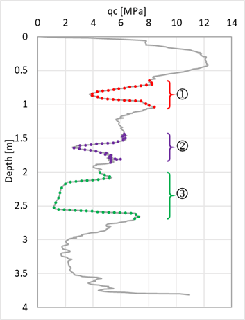
For location number 2 (depth of 1.45 to 1.85 m) the corrected q_c values are calculated as follows:

Upper part:

• < = 6.2 MPa
•  = 0.42
• Min TZ (Eq. 1) = 137 mm > depths in which the drop in  occurs, hence correction is needed
•  (Eq. 3) = 0.662



Lower part:

•  = 5.2 MPa
•  = 0.42
• Min TZ (Eq. 2) = 78 mm > depths in which the drop in  occurs, hence correction is needed

(a) (b)

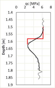
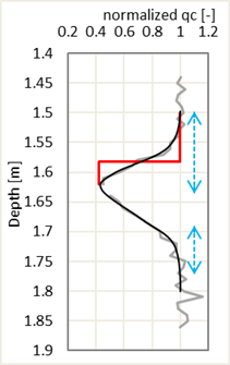
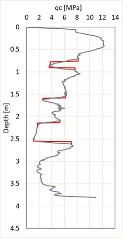
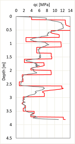
The recorded and corrected q_c values for location 2 (as numbered in Figure 7) are plotted in Figure 8(a), and the normalized q_c over the same depth in Figure 8(b). In the latter graph the min extent of TZs to make this method applicable are shown by blue dotted lines (Step I). The proposed corrections are plotted by red lines. The measured and normalized q_c graphs are simplified by black curve. Corrections of q_c at other depths were calculated in the same manner and presented in Figure 9(a).

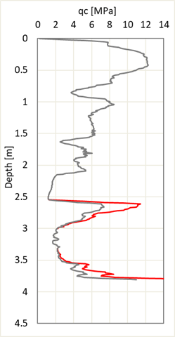
The same CPT graph is corrected for thin layer effect according to [7] (Boulanger and DeJong) and [5] (de Greef and Lengkeek) methods. Figure 9 compared the these corrections with the introduced method.

Boulanger and DeJong method considers the soil to be fully layered with sharp rises or drops at the borders instead of gradual changes from one layer to another. The soft-dense borders of de Greef and Lengkeek method are only where a coarse grained layer (I_c<2.6) is sandwiched between two fine grained layers (I_c>2.6). No correction is considered within layers with I_c below 2.6 even in case of rapid change in q_c.

(a) (b) (c)

Unlink Boulanger and DeJong method, the correction introduced here does not significantly increases or decreases the monitored q_c values, however, the soft-dense borders are among those captured by Boulanger and DeJong method.

4. Conclusions and Recommendations

From the outcomes of this study the following points can be concluded:

1. CPT test can sense a soft layer located ahead of its cone from a larger distance than when it is behind.
2. TZ is larger when CPT cone entered from a dense to a soft soil than the opposite order.
3. As per the conducted analyses, the CPT results in layered soils (e.g., TZ shape, or seem to be a function of stiffness ratio (R_s) rather than moduli of elasticity of the dense and soft soils individually.
4. Extension of TZ in dense soils above and below a soft layer is more function of R_s than soft layer thickness (h_s).
5. For thin, soft layers (here <300 mm) the measured q_c inside the soft layer cannot reach to the actual (or unaffected) q_c values. This gap is found to be a function of R_s and h_s.
6. A method is introduced in this paper to estimate the h_s and the actual q_c values inside and outside a soft layer embedded in dense soil from field data.
7. The proposed correction procedure must be repeated for every sharp increase or decrease in q_c.
8. In order to avoid human errors, this method is capable to be computerized.
9. In a future research work, CPT tests can be conducted in layered soils with known parameters (e.g., calibration chamber test) to evaluate the proposed method.

References

[1] T. Lunne, P. K. Robertson and J. M. Powell, “Cone penetration testing in geotechnical practice,” Blackie Academic & Professional, London, UK, 1997.
[2] D.D. Treadwell, “The influence of gravity, prestress, compressibility, and layering on soil resistance to static penetration,” Ph.D. thesis, University of California at Berkeley, Berkeley, USA. 1976.
[3] T.L. Youd, I. M. Idriss, R. D. Andrus, I. Arango, G. Castro, J. T. Christian, R. Dobry, W. D. L. Finn, L. F. Harder, M. E. Hynes, K. Ishihara, J. P. Koester, S. S. C. Liao, W. F. Marcusson, G. F. Martin, J. K. Mitchell, Y. Moriwaki, M.S. Power, P. K. Robertson, R. B. Seed and K. H. Stokoe, “Liquefaction Resistance of Soils: Summary Report from the 1996 NCEER and 1998 NCEER/NSF Workshops on Evaluation of Liquefaction Resistance of Soils,” Journal
[4] R.W. Boulanger, D. M. Moug, S. K. Munter, A. B. Price and J. T. DeJong, “Evaluating Liquefaction and Lateral Spreading in Interbedded Sand, Silt and Clay Deposits using the Cone Penetrometer,” Australian Geomechanics, vol. 51, no. 4, pp. 109-128. 2016.
[5] J.de Greef and H. J. Lengkeek, “Transition- and thin layer correction for CPT based liquefaction,” in Proceeding of Cone Penetration Testing Conference, Delft, the Netherlands, 2018, pp. 317-322.
[6] M.M. Ahmadi and P. K. Robertson, “Thin-layer effects on the CPT qc measurement,” Canadian Geotechnical Journal, vol. 42, no. 5, pp. 1302–1317, 2005. doi: 10.1139/t05-036 View Article
[7] R.W. Boulanger and J. T. DeJong, “Inverse filtering procedure to correct cone penetration data for thin-layer and transition effects,” in Proceeding of Cone Penetration Testing Conference, Delft, the Netherlands, 2018, pp. 25-44.
[8] F.S. Tehrani, M. I. Arshad, M. Prezzi and R. Salgado, “Physical modeling of cone penetration in layered sand,” Journal of Geotechnical and Geoenvironmental Engineering (ASCE), vol. 144, no. 1, pp. 04017101, 2018. doi: 10.1061/(ASCE)GT.1943-5606.0001809. View Article
[9] Z.Mlynarek, S. Gogolik and J. Poltorak, “The effect of varied stiffness of soil layers on interpretation of CPTU penetration characteristics,” Archives of Civil and Mechanical Engineering, vol. 12, pp. 253–264, 2012. View Article
[10] C.C. Hird, P. Johnson and G. C. Sills, “Performance of miniature piezocones in thinly layered soils,” Géotechnique, vol. 53, no. 10, pp. 885–900, 2003. View Article
[11] P.Q. Mo, A. M. Marshall and H. S. Yu, “Centrifuge modelling of cone penetration tests in layered soils,” Géotechnique, vol. 65, no. 6, pp. 468–481, 2015. View Article
[12] P.Q. Mo, A. M. Marshall and H. S. Yu, “Interpretation of cone penetration test data in layered soils using cavity expansion analysis,” Journal of Geotechnical and Geoenvironmental Engeering (ASCE), vol. 143, no. 1, 2017, doi: 10.1061/(ASCE)GT.1943-5606.0001577. View Article
[13] J.Walker and H. S. Yu, “Analysis of the cone penetration test in clay,” Géotechnique, vol. 60, no. 12, pp. 939–948b, 2010. View Article
[14] P.Van den Berg, R. De Borst and H. Huetink H., “An Eulerian finite element model for penetration in layered soil,” International Journal of Numerical and Analytical Methods in Geomechanics, vol. 20, pp. 865–886, 1996. View Article
[15] R.Vreugdenhil, R. Davis and J. Berrill, “Interpretation of cone penetration results in multilayered soils,” International Journal of Numerical and Analytical Methods in Geomechanics, vol. 18, no. 9, pp. 585–599, 1994. View Article
[16] P.D. Kiousis, G. Z. Voyiadjis and M. T. Tumay, “A large strain theory and its application in the analysis of the cone penetration mechanism,” International Journal of Numerical Analysis Methods Geomechanics, vol. 12, no. 1, pp. 45–60, 1988, doi: 10.1002/nag.1610120104. View Article
[17] M.M. Ahmadi, “Analysis of cone tip resistance in sand,” Ph.D. thesis, University of British Columbia, Vancouver, Canada, 2000.
[18] H.F. Schweiger, C. Fabris, G. Ausweger and L. Hauser, “Examples of successful numerical modelling of complex geotechnical problems,” Innovative Infrastructure Solutions, vol. 4, no. 1, 2018. doi: 10.1007/s41062-018-0189-5 View Article
[19] P.Jarast and M. Ghayoomi, “Numerical Modeling of Cone Penetration Test in Unsaturated Sand inside a Calibration Chamber,” International Journal of Geomechanics (ASCE), vol. 18, no. 2, pp. 04017148-1-13, 2018. doi: 10.1061/(ASCE)gm.1943-5622.0001052. View Article