1. Introduction

In recent decades, many civil infrastructures such as bridges, highways, and buildings have been subjected to increasing demands caused by traffic growth, environmental actions, and aging-related deterioration. Numerous bridges constructed more than half a century ago are now approaching or exceeding their design lifespans, raising growing concerns about structural safety, serviceability, and maintenance efficiency. These challenges highlight the urgent need for reliable and cost-effective assessment approaches to ensure the long-term performance and sustainability of critical infrastructure systems.

Structural Health Monitoring (SHM) integrates sensing technologies with computational modeling to evaluate and predict structural conditions in real time. Only sensing-based SHM faces challenges such as high cost, limited coverage, and incomplete data. Integrating SHM with the Finite Element Method (FEM) addresses these issues by providing a flexible numerical platform for simulating stress, deformation, and dynamic responses under various conditions. Through virtual sensing, FEM enables estimation of unmeasured responses, supporting digital-twin development for continuous monitoring and predictive maintenance.

In the finite element modeling of cable-stayed bridges, stay cables are typically idealized as single tension-only truss elements with reduced stiffness to account for sag effects. Although this approach offers simplicity and computational efficiency, it may be insufficient for model-based SHM, where accurate reproduction of the real dynamic behavior is essential to reliably assess current structural conditions and detect hidden damages [1]. Simplified modeling can cause discrepancies in the predicted cable forces, self-equilibrated shapes, and modal characteristics, reducing the fidelity of model validation with field data. Caetano [3] have investigated cable modeling schemes and sag formulations, but their findings were primarily based on numerical or laboratory studies without full-scale field validation.

Although many studies have explored the dynamic behavior of cable-stayed bridges, the combined effects of cable discretization and sag representation on the global modal characteristics of full-scale structures remain insufficiently quantified. Previous research, such as that by Caetano [3], mainly focused on simplified or small-scale models, leaving uncertainty about their influence on real bridge responses. To address this gap, this study investigates how cable discretization and sag representation affect the dynamic behavior of the full-scale Bhumibol Bridge I in Bangkok, Thailand. Field-measured vibration data are used for model validation, comparing finite element models with different cable element divisions and Ernst’s effective modulus. The results provide practical guidance for reliable FEM construction in SHM and digital-twin applications.

2. Basic theories and principles

2.1 Dynamic Behavior of Cable-Stayed Bridges

The dynamic behavior of cable-stayed bridges is governed by the complex interaction among three primary structural components: the deck, pylons(towers), and stay cables. The stay cables, serving as the main load-carrying members, transfer forces between the deck and pylons and play a dominant role in determining the global stiffness and vibration characteristics of the entire structure [2], [3]. Owing to their geometric slenderness, low damping, and high flexibility, cable-stayed bridges exhibit distinct dynamic responses that differ substantially from those of conventional beam or truss systems [4], [5]. Under dynamic excitations such as wind, traffic, or seismic loading, these bridges experience coupled motions that include vertical, lateral, and torsional vibrations of the deck, longitudinal movements of the pylons, and both in-plane and out-of-plane vibrations of the stay cables [6], [7].

These responses are highly nonlinear, mainly due to geometric nonlinearity caused by cable sag and large displacements, as well as material nonlinearity related to variations in axial tension and stiffness [8]–[10]. Since stay cables act as tension-only elements, their natural frequencies are strongly influenced by the axial force, self-weight, and unstrained length [11]. The vibration modes of cable-stayed bridges can generally be classified into three categories: [2] global modes representing the collective motion of the deck, pylons, and cables; [3] local cable modes dominated by the vibration of individual cables; and [4] hybrid modes that involve coupled motions between global and local components [12], [13].

Previous analytical and experimental investigations have emphasized that the coupling between cable vibration and the deck–pylon system significantly affects the overall dynamic behavior. Abdel-Ghaffar and Khalifa [14] showed that dividing each stay cable into multiple finite elements reveals numerous pure cable modes interacting with the deck and tower, resulting in complex hybrid responses that simplified single-element models cannot capture. Likewise, Caetano [3], through field and laboratory studies on the on a cable-stayed bridge in Spain, found that multi-element cable modeling generates a denser vibration spectrum with closely spaced global, local, and hybrid modes.

Accurate representation of these coupled dynamic characteristics is therefore essential for understanding the actual structural behavior of long-span cable-stayed bridges. Such understanding forms the analytical foundation for effective vibration analysis, design improvement, and SHM. of these large-scale systems.

2.2 Cable Modelling Approaches

The accuracy of finite element (FE) analysis for cable-stayed bridges largely depends on how stay cables are represented. As the main load-carrying and vibration-controlling components, stay cables strongly affect both global and local dynamic responses. Two principal modeling systems are generally adopted: the One-Element Cable System (OECS) and the Multi-Element Cable System (MECS) [3], [14].

In the OECS, each stay cable is modeled as a single truss element connecting the deck and pylon. The simplest configuration, referred to as the one-element linear model, assumes a straight cable with constant axial tension, neglecting self-weight and geometric sag effects. It employs the material’s full elastic modulus and provides high computational efficiency but often overestimates stiffness and natural frequencies, making it less suitable for detailed vibration studies.

A refined form of the OECS incorporates sag-induced flexibility through an equivalent elastic modulus derived from the Ernst formula [8]. This approach reduces the cable stiffness as a nonlinear function of its self-weight, span length, and horizontal tension, yielding a parabolic approximation of the sag curve. Studies such as Caetano [3] have shown that this refinement slightly lowers the predicted natural frequencies and improves agreement with measured modal data, providing a good balance between accuracy and efficiency.

The MECS, in contrast, divides each stay cable into multiple truss elements with distributed self-weight. This multi-node configuration enables the FE model to reproduce the catenary-shaped profile and to capture local cable vibrations as well as their coupling with deck and pylon motions. Abdel-Ghaffar and Khalifa [14] demonstrated that this discretization reveals numerous independent cable modes and complex coupled responses that simplified single-element systems cannot reproduce.

2.3 Effect of Sagging on Natural Frequency

In cable-stayed bridges, the sagging effect reduces the effective axial stiffness of stay cables, influencing both the global stiffness and dynamic characteristics of the structure. To represent this effect without resorting to nonlinear catenary modeling, Ernst [8] proposed an equivalent elasticity modulus that accounts for the reduction in stiffness due to sag. This approach has been widely adopted in practical bridge analyses for its balance between computational efficiency and accuracy. The equivalent modulus of elasticity is expressed as Eq.1

 =                                                              (1)

Where: E₀ is elastic modulus of the cable material, γ₀ is the weight per unit volume of the cable,L_x is the horizontal projection length of cable and σ₀ is initial stress in the cable due to the load increment

The reduction in the effective axial stiffness leads to a decrease in the natural frequencies of both individual cables and the overall bridge system. The magnitude of this reduction depends on the cable’s self-weight, tension level, and span length. For short, highly tensioned cables, the sagging effect is typically negligible; however, for long or lightly tensioned cables, it becomes significant and must be considered in dynamic analysis [2],[16].

2.5 Analysis of Cable Tension

The vibration and tension characteristics of stay cables play a fundamental role in defining the overall dynamic behavior of cable-stayed bridges. As long, slender, and tension-only members with negligible bending stiffness, stay cables can be reasonably modeled as taut strings subjected to distributed self-weight and axial tension [16]. The dynamic equilibrium of an infinitesimal cable segment leads to a one-dimensional wave equation that relates transverse vibration to axial force and mass per unit length.

Assuming small-angle motion, the relationship between cable tension and its natural frequency is derived Eq. 2 as:

(2)

where f_n is the natural frequency at vibration mode n, L is the cable length, T is the cable tension, and 𝜇 is the mass per unit length.

From this expression, the cable tension can be estimated based on Eq. 3.:

(3)

for the fundamental mode (n=1)

Expressing μ=ρA, where ρ is the material density and A is the cable cross-sectional area, gives in Eq. 4

(4)

This classical relationship forms the theoretical foundation of vibration-based cable-tension identification techniques widely used in SHM [2], [3]. By measuring the fundamental frequency f₁ from field vibration data typically obtained using accelerometers or Fiber Bragg Grating (FBG) sensors [21] the in-situ cable tension can be estimated indirectly without the need for load cells.

Although this vibration-based method is simple and computationally efficient, several studies [18] have reported that neglecting bending stiffness, boundary constraints, and environmental influences may introduce errors of up to 10 %. To overcome these limitations, advanced identification algorithms have been developed. Li et al. [18] proposed an Extended Kalman Filter (EKF)-based method for estimating time-varying cable tension from measured accelerations, achieving high robustness in numerical and laboratory tests. Similarly, Yang et al. [20] introduced a Blind Source Separation (BSS) technique capable of extracting instantaneous cable-tension variations from mixed ambient vibration data with improved accuracy.

In the present study, the fundamental frequency–tension relationship is employed to estimate the in-situ tension of stay cables in the Bhumibol Bridge I based on field-measured vibration data. The derived tension values are incorporated into the finite element model to examine their influence on global stiffness, modal frequencies, and the interaction between cable tension and sag effects, contributing to a more reliable model-based SHM framework for long-span cable-stayed bridges.

3. Methodology and Finite Element Model Development

3.1 Research Framework

The research framework is divided into three phases, as illustrated in Figure 1, Phase A for model construction, Phase B for field measurement, and Phase C for validation and analysis. This process provides a systematic approach to develop, calibrate, and validate the FEM of the Bhumibol Bridge I.

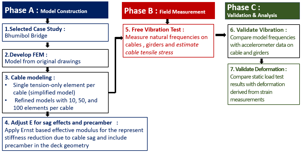
A detailed finite element model (FEM) of the Bhumibol Bridge I was developed from design drawings, focusing on stay cables that govern global stiffness and vibration behavior. The baseline model used single truss elements per cable, while refined models with 10, 50, and 100 elements captured curvature and higher vibration modes. The Ernst effective modulus represented effect and precamber was incorporated into the deck geometry to reflect the initial cambered configuration during construction. Free vibration tests under ambient traffic and wind provided field data for calibration. The final FEM was validated against measured natural frequencies, mode shapes, and static responses.

3.2 Overview of the Target Bridge

The target bridge of this study is the Bhumibol Bridge I, a cable-stayed bridge crossing the Chao Phraya River in Bangkok, Thailand (Figure 2). Opened in September 2006, it consists of a 326 m composite main span and 125 m post-tensioned concrete box girder side spans. The deck is supported by two 152 m-high diamond-shaped reinforced concrete towers and four side-span piers. Fixed connections between the deck, towers, and piers are made of homogeneously stressed concrete, with expansion joints provided at both ends of the side spans.

(a) General view of the Bhumibol Bridge I
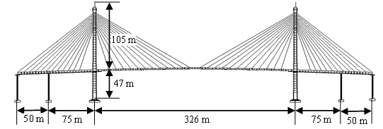(b) Bridge dimensions

3.3 Material Properties and Cable Modeling

The finite element model of the Bhumibol Bridge I uses structural steel for the girders and stay cables, and reinforced concrete for the pylons and deck, as summarized in Tables 1 and 2.

Table 1. Gerneral Material Properties

Name	Property	Value	Unit
Girders (Structural Steel)	Young’s modulus	2.10 × 10⁸	kN/m2
	Density	78.50	kN/m3
	Poisson’s ratio	0.3	-
Pylons & deck (Reinforce Concrete)	Young’s modulus	3.17 × 10⁷	kN/m2
	Density	23.63	kN/m3
	Poisson’s ratio	0.2	-
Asphalt	Density	24.50	kN/m3

Table 2. Cable Properties

Property	Value	Unit
Diameter	0.00157	m
Tensile strength	1.86 × 106	kN/m2
Cross-sectional area	1.50 × 10-4	m²
Mass per meter	0.001147	kN/m
Modulus of elasticity	1.95 × 108	kN/m²

In the finite element model, stay cables were modeled as tension-only elements. Eight scenarios were analyzed to examine the effects of discretization and sag (Table 3). Two approaches were used: the linear elastic modulus (E₀) without sag correction and the Ernst effective modulus (Eᵣₙₛₜ) accounting for sag-induced stiffness reduction (Eq. 1). Each cable was idealized as a straight line between anchorage points (see Figure 3).

Table 3. Cable Modeling Scenarios

Case	Modulus of Elasticity	No. of Elements
1 (Base model)	E0(100%)	1 element (original)
2	E0(100%)	10 elements
3	E0(100%)	50 elements
4	E0(100%)	100 elements
5	Ernst	1 element
6	Ernst	10 elements
7	Ernst	50 elements
8	Ernst	100 elements

(a) 1- element cable
(b) 10- element cable
(c) 50- element cable
(d) 100- element cable

3.4 Instrumentation and Sensor Layout

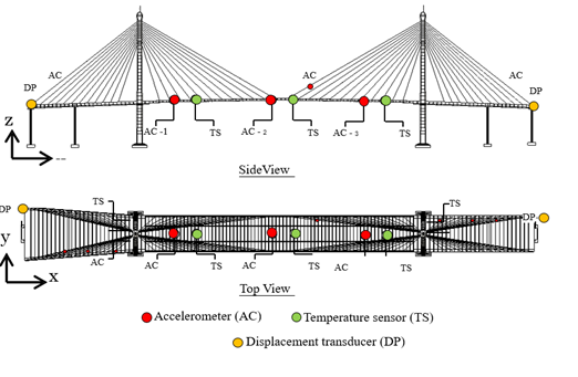
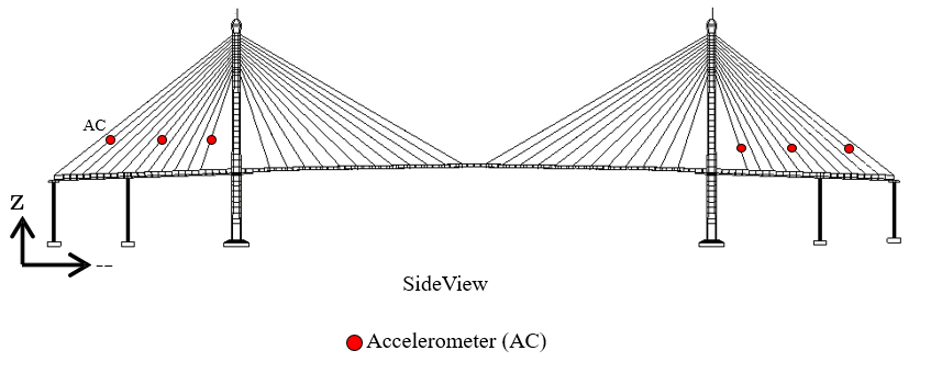
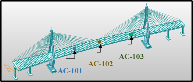
     Field measurements on the Bhumibol Bridge were conducted in two phases: the initial campaign in May 2014 and an upgraded system in September 2025, as shown in Figures 4 and 5. In 2014, a monitoring system was installed to collect baseline dynamic data. Accelerometers (AC, 50 Hz) on the main girder and the longest stay cables recorded vibration responses, while temperature sensors (TS) and displacement transducers (DP) measured environmental effects and global deflections for initial modal identification and model validation.

The 2025 campaign introduces an enhanced SHM system. Selected stay cables, including eight in the back span, are equipped with high-sensitivity accelerometers operating at 100 Hz to capture detailed vibration responses for advanced dynamic analysis and model validation.

3.6 Resonant Frequencies and Mode Shapes

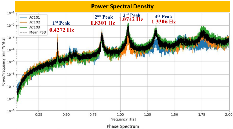
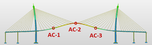
The resonant frequencies were identified from peaks in the power spectral density (PSD) of the deck’s vertical acceleration (Figure 6), computed from five-minute measurement segments (15,000 data points each). The identified peaks corresponding to the first four resonant frequencies are illustrated in Figure 7.

4.Finite Element Analysis

4.1 Modal Analysis of the Initial FE Model

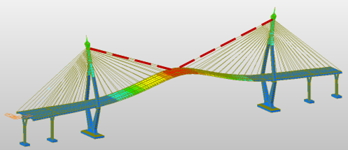
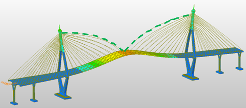
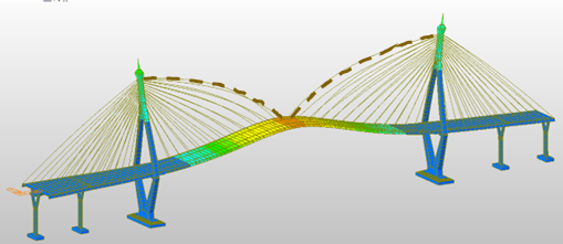
The finite element model of the Bhumibol Bridge I was developed from original design drawings in MIDAS Civil. Modal analysis was performed to determine natural frequencies and mode shapes, with stay cables modeled as single tension-only elements. Boundary conditions assumed fixed pylons, rigid deck connections, and pinned cable ends. The first four FE mode shapes are presented in Figure 8, and the comparison with field-measured frequencies is summarized in Table 4.

Table 4 Natural frequencies comparison between FE model and field measurement

Model	FE Model	Field Measurement (Hz)	Different (%)
1st	0.46482	0.4272	8.81%
2nd	0.87063	0.8301	4.88%
3rd	1.12337	1.0742	4.58%
4th	1.35933	1.3306	2.11%

(a) 1^st peak (0.46482 Hz)
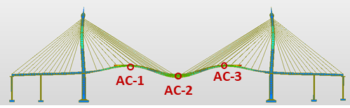(b) 2^nd peak (0.870631 Hz)
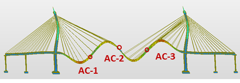(c) 3^rd peak (1.12337 Hz)
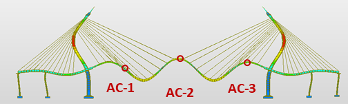(d) 4^th peak (1.35933 Hz)

4.2 Cable Modeling Scenarios

To improve accuracy, refined models with 10, 50, and 100 elements per cable were developed to account for distributed self-weight and realistic deformation behavior. The results show a consistent trend across the first four bending modes.

At the first mode, the results show that increasing the number of elements enhances the representation of cable curvature and local flexibility. However, the calculated frequency slightly increases when the cable is divided, and shows almost no change between 50 and 100 elements, as illustrated in Figure 9.

(a) 1 element cable divided, f = 0.46482 Hz

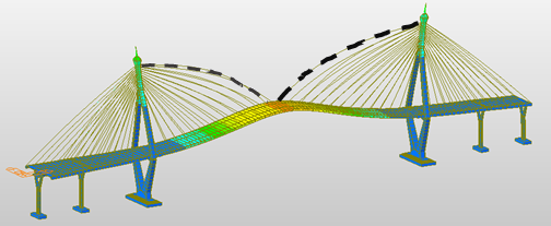
(b) 10 element cable divided, f = 0.465787 Hz

(c) 50 element cable divided, f = 0.465804 Hz

(d) 100 element cable divided, f = 0.465802 Hz

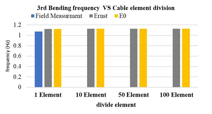
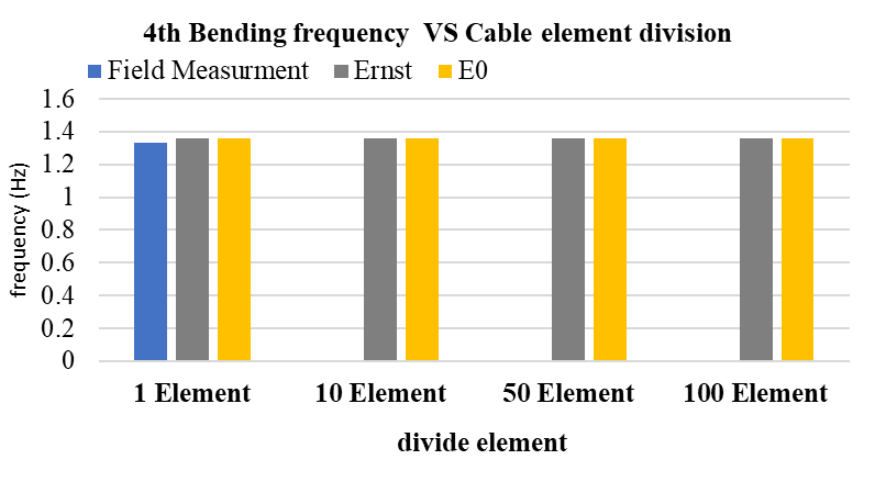
The frequency results for different cable modelling scenarios compared with field measurements for the 1st–4th modes, the calculated frequencies slightly increase when the cable is divided, and show almost no change between 50 and 100 elements, as shown in Table 5.

Table 5 Comparison of field-measured and FE-calculated natural frequencies for different cable element divisions

Mode	Field (Hz)	FE Analysis Result (E0): f(Hz)
		1 element	10 element	50 element	100 element
1st	0.4272	0.4648	0.4657	0.4658	0.4658
2nd	0.8301	0.8706	0.8753	0.8757	0.8757
3rd	1.0742	1.1233	1.1282	1.1277	1.1258
4th	1.3306	1.3593	1.3591	1.3613	1.3614

The trend of frequencies shows a slight increase beyond 10 elements and remains nearly unchanged after 50 to 100 elements, as shown in Figure 10. This stabilization reflects numerical convergence, where additional discretization no longer affects the cable’s stiffness representation. Beyond this point, the finite element mesh becomes sufficiently refined to capture the cable’s geometric nonlinearity and self-weight effects, resulting in consistent natural frequencies regardless of further element division.

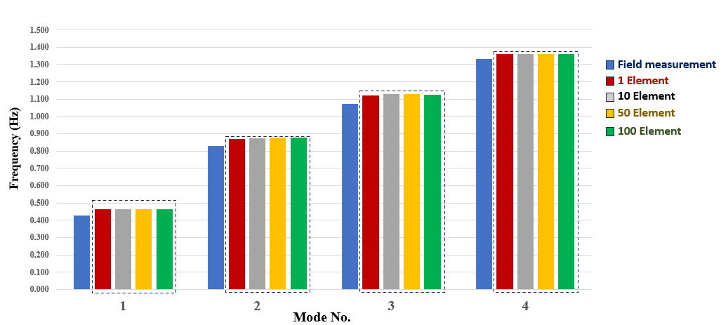
The slight increase in natural frequencies with finer cable element division occurs because multi-element models more accurately capture the cable’s curvature and flexibility, leading to a more realistic stiffness distribution. Beyond about 50 elements, the frequencies converge as the mesh becomes sufficiently refined to represent the cable’s self-weight and geometric nonlinearity, resulting in negligible changes in overall stiffness and dynamic response.

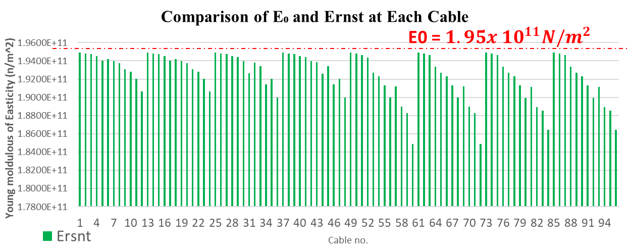
4.3 Equivalent Modulus by Ernst Formula

The stay cables were modeled with a nominal modulus of E₀=1.95x10¹¹ N/m².Considering sag effects, the equivalent modulus was derived from the Ernst formula (Eq. 3), accounting for self-weight, length, and initial tension. As shown in Figure. 11–12, the equivalent values are up to 5% lower, providing a more realistic dynamic representation.

The reduction in equivalent modulus becomes more pronounced in longer cables, as the increased sag due to self-weight reduces the effective axial stiffness. This behavior reflects the geometric nonlinearity of the cable, where a portion of the tensile force is consumed to support its own weight rather than resisting dynamic deformation. Consequently, longer and more flexible cables exhibit slightly lower equivalent stiffness and natural frequencies compared to shorter ones.

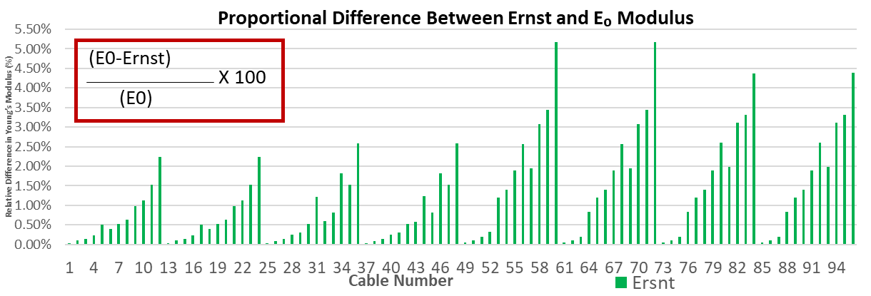
The decrease in equivalent modulus with longer cables occurs because greater sag consumes part of the tensile force to support self-weight, reducing effective axial stiffness. This geometric nonlinearity leads to slightly lower stiffness and natural frequencies, indicating that the Ernst-modulus approach realistically represents stiffness variation among cables of different lengths.

4.4 Comparison E_rnst with Constant E₀ Assumption

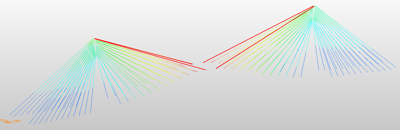
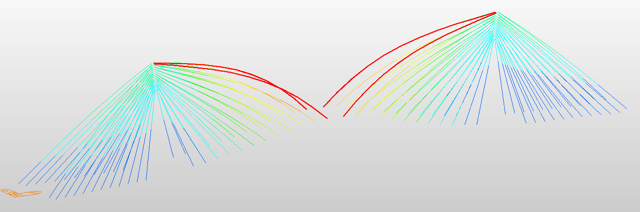
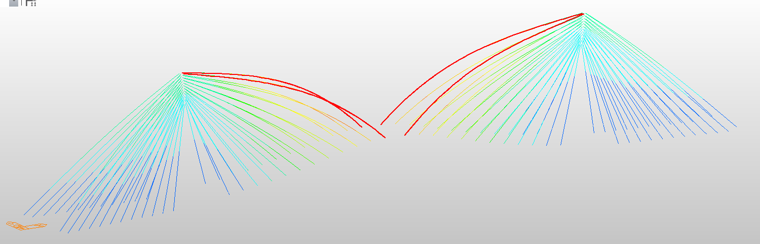
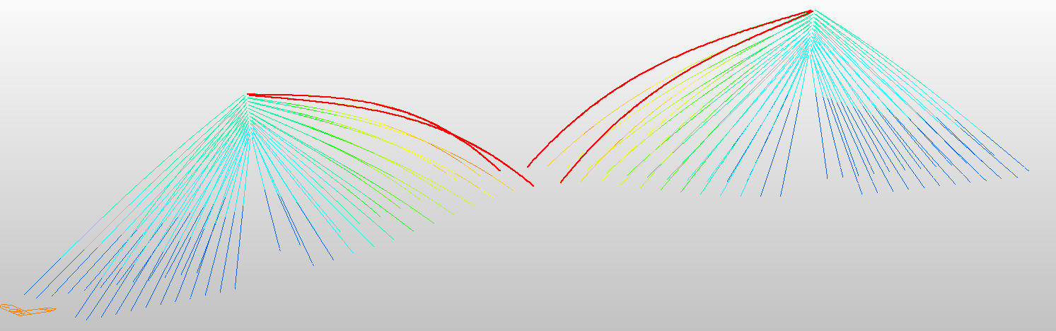
To evaluate the influence of the sag effect, the results from the Ernst-modified modulus (Ernst) were compared with those obtained using the constant elastic modulus (E₀). As shown in Figure 13, the use of the Ernst modulus slightly lowers the calculated natural frequencies compared to E₀, reflecting the stiffness reduction due to cable sag.

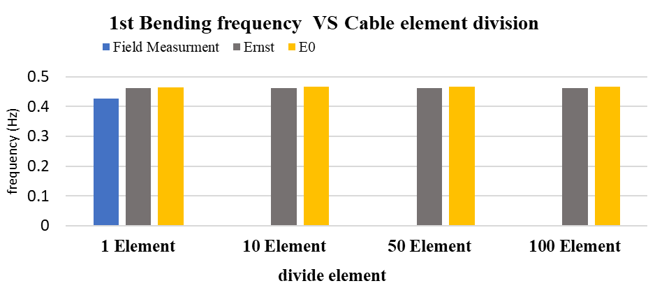
(a) 1^st bending mode vs. cable element division

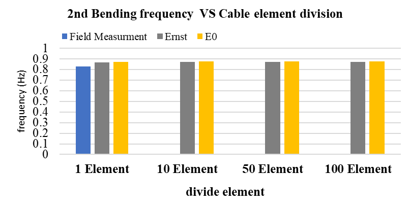
(b) 2^nd bending mode vs. cable element division

(c) 3^rd bending mode vs. cable element division

(d) 4^th bending mode vs. cable element division

The slight reduction in natural frequencies using the Ernst-modified modulus reflects the sag-induced stiffness reduction of the cable system. This results in a more realistic global stiffness, improving the agreement of the main structural bending modes with the field-measured frequencies compared to the constant E₀ assumption, thereby enhancing the accuracy of the dynamic analysis.

4.5 Cable Frequency Measurement and Tracking Cable Modeling

Cable frequency measurements were conducted on selected stay cables of the Bhumibol Bridge I (Figure 4 and 5) .Accelerometers were installed on short, middle, and long cables in the back span and the longest cable in the main span to record ambient vibrations. The identified FFT peak frequencies, used for FE model validation, are summarized in Table 6

Table 6 Representative FFT peak frequencies of selected stay cables

Cable No.	Type of Cable	1St Mode (Hz)	2nd Mode (Hz)
MN4B1E	Short	1.860	3.721
MN4B6E	Medium	1.160	2.323
MN4B11E	Long	0.781	1.546
MN3B1W	Short	1.873	3.691
MN3B6W	Medium	1.219	2.434
MN3B11W	Long	0.786	1.556
MN4M12W	Longest	0.621	0.887

For tracking the short cable shows consistent mode shape across all cases, with frequencies slightly increasing as element division refines. The single-element model fails to capture the measured behaviour or realistic mode shape as shown in Figure 14.

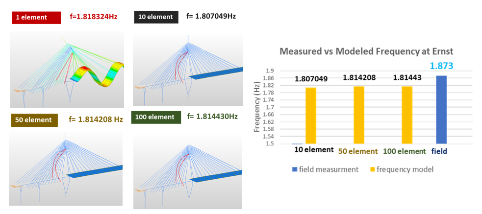
A similar trend is observed for the first modal frequency of cable where the overall frequency decreases with increasing cable length. Increasing the number of cable elements slightly raises the frequencies in both girder- and cable-dominated modes. However, for the second mode of long stay cables, the frequencies remain nearly constant beyond 50 elements, while the mode shape patterns become smoother.

These results show that finer cable discretization improves modal accuracy by better representing curvature and flexibility. The slight frequency increase reflects reduced artificial stiffness in coarse models, while convergence beyond 50 elements indicates sufficient refinement to capture the cable’s true dynamic behavior.

4.6 Effect of Precamber

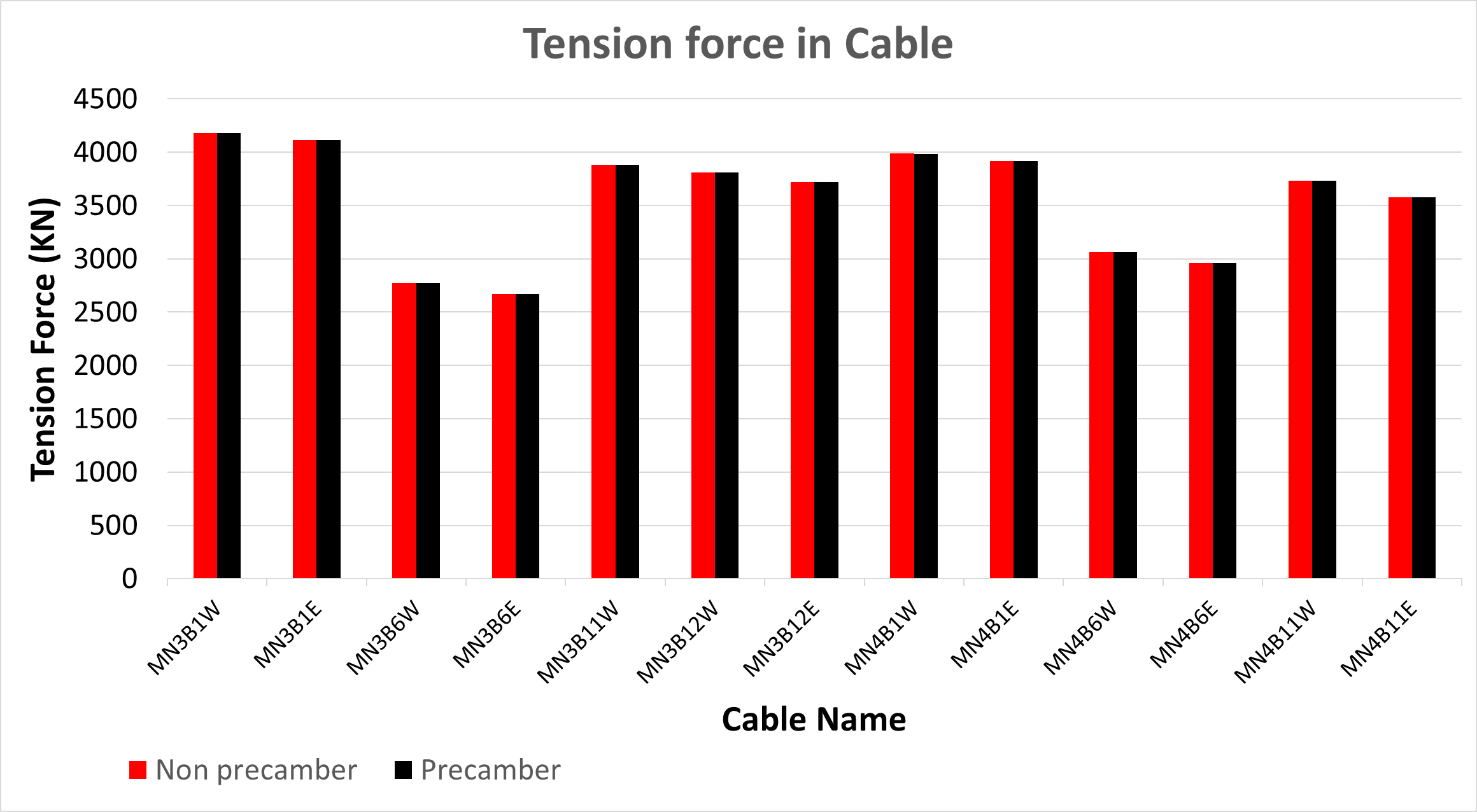
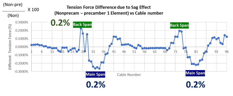
The influence of precamber on cable forces was examined using FE models with and without precamber based on the Ernst-modified modulus. As shown in Figures 15–16, the overall force distribution remains nearly identical, with differences within ±0.2% and slightly higher sensitivity in the back- and main-span regions. Although minor, precamber slightly modifies the tension distribution, which may affect the bridge’s vibration characteristics.

Figure 15 Tension force distribution in cables with and without precamber using the Ernst-modified modulus.

The effect of precamber on modal responses was evaluated using the Ernst-modified modulus with 100 cable elements. As shown in Table 7, the natural frequencies remain close to field data, with precamber slightly reducing frequencies in girder-related modes (1st and 2nd). The mode shapes also align well with field observations, indicating that precamber improves the accuracy of the predicted dynamic behavior

The slight frequency reduction in girder-related modes results from precamber altering the initial geometry and stiffness distribution, slightly lowering global rigidity. This adjustment produces frequencies closer to field data, confirming that including precamber improves the realism of the dynamic response prediction.

Table 7 Comparison of field and FE frequencies with/without precamber (Ernst modulus, 100 elements)

Mode	f (Hz)	Ernst 100 element Non precamber		Ernst 100 element precamber
	Field Measurement	f (Hz) Ernst model	Different from filed (%)	f (Hz) Ernst model	Different from filed (%)
1st	0.4272	0.4617	8.09%	0.4614	8.01%
2nd	0.8301	0.8714	4.98%	0.8709	4.92%
3rd	1.0742	1.1258	4.81%	1.1264	4.87%
4th	1.3306	1.3598	2.20%	1.3627	2.41%

4.7 Validation of FE Model with Field Data

The comparison between field measurements and modeling results in Table 8 shows that when using 100 elements per cable, the natural frequency gradually decreases as the cable length increases. The short cable in the back span shows a frequency difference of about 3–5% between the numerical and measured results. The middle cables show the largest difference (15–16%), while for the long and longest cables, the differences decrease to 7% and 1%, respectively. Moreover, when considering the first peak mode (single curve), the overall frequency trend consistently decreases with increasing cable length, showing a clear relationship between cable length and vibration characteristics.

The decreasing frequency trend with increasing cable length occurs because longer cables experience greater sag and lower axial stiffness. Short cables remain taut and stiffer, producing higher frequencies and smaller discrepancies. The larger differences in middle cables, where the modeled frequencies are lower than the measured values, may be due to underestimation of boundary stiffness or pretension, making these cables less sensitive to the assumed modeling conditions.

Table 8 Comparison of field measurements and modeling results for cable vibration frequencies (100-element cable model)

Cable No.	Type of Cable	Field measurement f(Hz)	FE Modeling (Hz)	Different from field measurement (%)
MN4B1E	Short	1.860	1.7728	5
MN3B1W	Short	1.873	1.8144	3
MN4B6E	Medium	1.166	0.9884	15
MN3B6W	Medium	1.219	1.0294	16
MN4B11E	Long	0.781	0.7123	9
MN3B11W	Long	0.786	0.7265	8
MN4M12W	Longest	0.621	0.6263	1

References

[1] K. Tiprak, K. Takeya, and E. Sasaki, “Integrated neural networks–Particle Swarm Optimization for probabilistic finite element model updating: application to a prestressed concrete girder bridge,” Structure and Infrastructure Engineering, pp. 1–35, 2024. View Article
[2] H. Zui, T. Shinke, and Y. Namita, “Practical formulas for estimation of natural frequencies of cable-stayed bridges,” Journal of Structural Engineering, American Society of Civil Engineers, vol. 122, no. 4, pp. 382–390, 1996. View Article
[3] E. Caetano, Cable Vibrations in Cable-Stayed Bridges, London: Taylor & Francis, 2007.
[4] Y. L. Xu and Y. X. Yu, “Dynamic behavior of cable-stayed bridges under earthquake excitation,” Earthquake Engineering and Structural Dynamics, vol. 26, no. 6, pp. 603–619, 1997.
[5] J. M. W. Brownjohn and P. Q. Xia, “Dynamic assessment of long-span bridges by continuous vibration monitoring,” Journal of Bridge Engineering, American Society of Civil Engineers, vol. 5, no. 4, pp. 293–303, 2000.
[6] X. Chen and A. Kareem, “Coupled dynamic analysis and aerodynamics of cable-stayed bridges,” Journal of Structural Engineering, American Society of Civil Engineers, vol. 129, no. 5, pp. 615–625, 2003.
[7] W. X. Ren and A. Chen, “Finite element simulation of vibration and damage detection of cable-stayed bridges,” Engineering Structures, vol. 32, no. 2, pp. 593–604, 2010.
[8] R. Ernst, “Der E-Modul von Seilen unter Berücksichtigung des Durchhanges,” Bauingenieur, vol. 40, pp. 52–55, 1965.
[9] Y. X. Xia and C. S. Cai, “Practical considerations for modeling cable-stayed bridges,” Journal of Bridge Engineering, American Society of Civil Engineers, vol. 16, no. 1, pp. 54–62, 2011.
[10] H. Lee and J. Lee, “Dynamic characteristics of cable-stayed bridges considering geometric nonlinearities of stay cables,” Journal of Sound and Vibration, vol. 269, no. 3–5, pp. 1031–1043, 2004.
[11] H. M. Irvine, Cable Structures, Cambridge, MA: MIT Press, 1981.
[12] E. Caetano, A. Cunha, and F. Moutinho, "Modal analysis of cable-stayed bridges: Experimental and numerical investigations," Journal of Bridge Engineering, American Society of Civil Engineers, vol. 5, no. 4, pp. 293–302, 2000. View Article
[13] S. Zivanovic and A. Pavic, "Vibration serviceability of footbridges under human-induced excitation: Literature review," Journal of Sound and Vibration, vol. 279, no. 1–2, pp. 1–74, 2006. View Article
[14] A. M. Abdel-Ghaffar and M. A. Khalifa, "Importance of cable vibration and damping in dynamics of cable-stayed bridges," Journal of Engineering Mechanics, American Society of Civil Engineers, vol. 117, no. 11, pp. 2571-2589, 1991. View Article
[15] A. R. Chen, Y. X. Xia, and C. S. Cai, "Equivalent modulus for modeling sag effect of stay cables and its application in bridge dynamic analysis," Journal of Bridge Engineering, American Society of Civil Engineers, vol. 5, no. 2, pp. 134–142, 2000. View Article
[16] J. T. Kim and J. H. Park, "Finite element model updating of a cable-stayed bridge considering sag and bending stiffness of cables," Engineering Structures, vol. 59, pp. 439–455, 2014. View Article
[17] X. He and G. Fu, "Modal analysis and parametric study of cable vibration for cable-stayed bridges," Journal of Bridge Engineering, American Society of Civil Engineers, vol. 6, no. 6, pp. 497–505, 2001. View Article
[18] M. Geier and R. Flesch, "On the determination of cable forces by vibration measurements considering bending stiffness and boundary conditions," Engineering Structures, vol. 197, Article ID 109380, 2019. View Article
[19] H. N. Li, D. S. Li, and G. B. Song, "Recent applications of vibration-based damage identification methods to civil engineering structures," Journal of Civil Structural Health Monitoring, vol. 1, no. 1–2, pp. 17–36, 2010. View Article
[20] Y. Yang, Y. Zhang, and S. Li, "Identification of time-varying cable tension using blind source separation of measured vibration responses," Smart Materials and Structures, vol. 21, no. 8, Article ID 085022, 2012. View Article
[21] W. Zhu, Y. Guo, J. Yu, and L. Liu, "Measurement of cable force through a fiber Bragg grating sensor," Sensors, vol. 22, no. 21, p. 8203, 2022. View Article